Exam 1

Question 1

statistics

Answer 1

scientific analysis of data in whose generation randomness/chance played some part

necessary to handle data since math isn’t enough because randomness is unavoidable in science

ex. how does the weight of a baby depend on its age? how does BP depend on genetics? Monty Hall Problem.

Question 2

direction: probability is _____, while statistics is ______

Answer 2

prob is deductive. starts with if statement… then some prob calculation about data. ->

stat is inductive, starts with data and relevant prob calcs to make a statement about reality. <-

zig-zag relationship

Question 3

probability notation

Answer 3

events: A, B, …

probability that event A will happen = Prob(A)

Question 4

derived events

Answer 4

A u B: union, A or B or both

A n B: intersection, both

Question 5

mutually exclusive events

Answer 5

F and G are mutually exclusive if they cannot happen in the same experiment. If F, G…H are mutually exclusive, P(F u G u … H) = Prob(F) + Prob(G)… + Prob(H).

Question 6

independence

Answer 6

F and G are independent iff the probability of their intersection, Prob (F n G) = Prob(F) x Prob(G).

We often assume independence.

When F and G are independent, the conditional probability formula cancels out by filling in the prob of union equation. AKA F and G are independent if G having occured doesnt change the prob that F occurs.

If two events are mutually exclusive, they cannot be independent The oppositie may or may not be true.

Question 7

conditional probabilities

Answer 7

the probability that F occurs given that G has occured

Prob (F | G) = Prob(F n G) / Prob(G)

Question 8

discrete and continuous random variables

Answer 8

concept of the mind numbers

discrete RV: a conceptual and numerical quantity which in some future experiment will take on or other of a discrete set of values with known or unknown probabilities (only take one or other of a set of discrete values, usually 0, 1, 2, 3…)

continuous RV: can take any value in a continuous range of values RVs are written with upper case letters.

Question 9

data

Answer 9

the observed values of RVs after the relevant experiment has been carried out. written with lower case letters.

Question 10

presenting probabilities

Answer 10

tableau with possible values of X and probabilities of X (probs sometimes known, sometimes unknown)

or graph (known)

Question 11

parameters

Answer 11

some usually unknown numerical value, denoted with a greek letter

Question 12

discrete RV notation

Answer 12

Prob( X = vi) is a shorthand for “the prob that, once the exp is carried out, the observed value x of X will be vi”

Question 13

conditions for binomial distribution

Answer 13

1) we conduct a fixed number of trials
2) there are only two possible outcomes on each trial. We call these success and failure
3) the outcomes of the various trials are independent
4) the probability of success, θ, is the same on all trials RV of interest is the number of successes, X, in n trials

Question 14

third method of presenting probability distribtuion

Answer 14

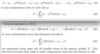
(n x) is the # of orderings in which there are x successes in the n trials = n! / (n-x)!x!

the second part is the probability of getting x successes in n trials in a specified order

Question 15

mean

Answer 15

NOT AN AVERAGE, a parameter, denoted μ, for binomal distribution, μ = nθ

it is the balance point (where areas under the curve are equal)

mean is a proberty of the being

MUST KNOW LONG AND SHORT FORMULAS FOR MEAN

Question 16

average

Answer 16

calculated from data, estimates the mean, denoted x̄

precision depends on sample size and the propoerties of the RV X̄, the concept of the mind average before we roll the die

Question 17

variance

Answer 17

always denoted σ²

it is a meausre of the spread outness of the probability distribution of X relative to the mean of X

for binomial distribution var of X = nθ (1 - θ)

important because the precision of x̄ as an estimate of μ depends on the variance of the RV X̄

MUST KNOW LONG AND SHORT FORMULAS FOR VARIANCE

Question 18

complementary events

Answer 18

A^c is the event that A did not happen.

Prob (A^c) = 1 - Prob (A)

Question 19

standard deviation

Answer 19

σ = sqrt (variance of X)

often more useful in practice than variance bc its not in squared units

Question 20

deductive and inductive example

Answer 20

if a newborn is equally likely to be a boy as a girl, then in a well-conducted, representative, unbiased (WRU) sample of 40,000 newborns, then probability of getting between 19800 and 20200 boys is .95

In a WRU sample of 40K newborns we saw 20288 boys. Possible reasonable stat induction is that is is not equally likely that a newborn is a boy as a girl.

Question 21

probability of union equation

Answer 21

P(F u G) = Prob(F) + Prob(G) - Prob( F n G)

Question 22

3 main activities of stat

Answer 22

1) estimating the value of a mean using an average
2) assesing the precesion of the estimate
3) testing hypotheses about a mean or multiple means

Question 23

theory for many RVs is necessary because

Answer 23

we need it to make proper statistical inferences about data x₁…x_n

Question 24

n

Answer 24

notation for sample size

DIFFERENT from k

for a die, k = 6 (6 possible values when you roll it)

n = # of times you will roll it

Question 25

iid

Answer 25

independently and identically distrubuted

we assume iid unless stated otherwise

Question 26

T_n

Answer 26

mean of T_n = nμ

variance of T_n = n σ²

MUST KNOW ABOVE FORMULAS

Question 27

X̄

Answer 27

mean of X̄ = μ

variance of X̄ = σ²/n

MUST KNOW ABOVE FORMULAS

(larger n -> smaller variance. ex. JMP exercise)

relevance to stat: if we estimate the numerical value of a mean μ by a data average x̄, the precesion of the estimate depends on the variance σ²/n of X̄. this can help us make stat inductions.

Question 28

differences

Answer 28

D = X₁ - X₂

an RV

mean of D = 0 (or = μ₁ - μ₂)

variance of D = 2 σ² (or = σ₁² + σ₂²)

MUST KNOW ABOVE FORMULAS

Question 29

proportion of successes (P)

Answer 29

need to use P to make a fair comparison between different sample sizes

If X is the # of successes in n binomial trials, P = X/n

mean of P = θ

variance of P = θ(1 - θ) /n

MUST KNOW MEAN AND VARIANCE OF P

Question 30

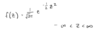
density function

Answer 30

for continuous RVs we allocate probabiliites to ranges of values using the RV’s density function

Question 31

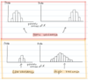
normal distribution

Answer 31

the continuous RV X has a normal distribution with mean μ and variance σ² if its density function is as follows in the pic

creates a bell shaped curve

not one single distribution but a family of them

sums, averages and differences of iid RVs all have a normal distribution

Question 32

Z

Answer 32

a normal distribution of specific focus with μ = 0 and σ² ​= 1

probabilities are evaluated using a chart

Question 33

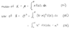
mean and variance of a continuous RV

Answer 33

Question 34

standardization procedure or Z-ing

Answer 34

(X - μ) / σ ​= Z

Question 35

two standard deviation rule

Answer 35

gives you a 95% confidence interval

approximated to 2 from Z < 1.645 and -1.96 < Z < 1.96

often used in stat to make probability statements about the RVs sum, average, X, and P

Question 36

the central limit theorem

Answer 36

the reason we consider normal distribution in detail

says that if the RVs X₁…X_n are iid, no matter the probability distribution of those RVs, the average X̄ and sum T_n both have approximately normal distributions and the approximation gets more accurate as n increases

allows us to use magic formulas with the many stat procedures that deal with n binomial trials

Question 37

die graphs

Answer 37

show 5 things:

1 + 2) formulas for mean and variance of sum

3 + 4) formulas for mean and variance of average

5) central limit theorem: sums and averages have approx normal distributions

Question 38

estimate of θ

Answer 38

we estimate θ by proportion of successes

p = x/n <- this is the estimator

p is an unbiased estimate of θ aiming at the right target

the properties of this estimate depend on the properties of the RVs (the mean of P = θ)

Question 39

how accurate is the estimate of θ?

Answer 39

depends on the variance θ(1 - θ) /n of P

flip the 2SD rule using the 10 yard rule and substitute θ for p (since p is an estimate of θ) to create the 95% confidence interval

Question 40

conservative 95% confidence internval for p

Answer 40

derived from the idea that p( 1 - p) is about equal to 1/4

its approximation is always a bit wider than if you use the usual interval

Question 41

margin of error

Answer 41

= 1/ sqrt(n)

can be used to determine n (and how precise the poll is)

larger n -> more precise but more expensive

if you want to be twice as accurate, you need four times the sample size

Question 42

99% confidence interval

Answer 42

papers often don’t specify if their margin of error was determined by the 95 or 99% confidence interval

Question 43

JMP

Answer 43

proof of principle that the average as an estimator gives a good idea of the mean

Question 44

conservative 99% confidence interval

Answer 44

Question 45

fair die rolled once

Answer 45

the mean of the number to turn up is 3.5 and the variance of the number to tun up is 35/12

Question 46

probabilities for X when flipping a coin and n = 2, X = # of heads

Answer 46