National income and price determination Flashcards
The relationship between the quantity of real GDP demanded and the price level is called ________ Demand.
Aggregate
Explanation
Aggregate Demand (AD) is a schedule, graphically represented as a curve, that shows the total amount of goods and services that consumers, businesses, governments, and foreigners will want to purchase at each possible price level.
1) The quantity of real GDP demanded is the total amount of final goods and services produced in a country that people (C), businesses (I), governments (G), and foreigners (X) plan to buy in a given period of time and at a given price level.
The quantity of real GDP demanded is:
Y = C + I + G + X
The AD (Aggregate Demand) curve slopes ____.
down
Explanation
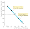
The downward slopes indicates that the lower the price level, the larger real domestic output will be purchased. The AD curve slopes downward for two reasons: Wealth effect and Substitution effects.

The tendency for increases in the price level to lower the purchasing power of assets of financial assets and reduce total spending in the economy is call the _____ effect.
Wealth
Explanation
Spending is less because the rise in prices will make some people less wealthy and they will spend less on consumption expenditure. The opposite holds true if prices decrease.

The ____________ effect on Aggregate Demand occurs when people change consumption between today and tomorrow and between domestic goods and services and foreign goods and services.
Substitution
Explanation
When current prices change it does not affect future prices so consumers put off buying today in favor of waiting for optimal conditions in the future. Likewise, when price levels in one country change it does not mean that price levels in other countries change, thus people substitute the less expensive foreign goods and services for higher priced domestic ones.

A change in any influence on spending plans other than the price level _____ the aggregate demand curve.
shifts
Explanation
A change in price usually means you just move up or down along the demand curve. However, a non-price influence on spending results in a shift of the entire demand curve.
1) The AD Curve shifts as a result of changes in expectations, fiscal and monetary policy, and the world economy.

Expected changes about jobs and incomes, inflation, and ____ affect spending plans and will shift the AD Curve.
profits
______ policy is the government’s attempt to influence the economy by setting and changing taxes, transfer payments, and expenditures on goods and services.
Fiscal
Explanation
Fiscal policy changes will shift the AD (Aggregate Demand) curve.
________ policy is the government’s attempt to influence the economy by setting and changing interest rates, the exchange rate, and the quantity of money.
Monetary
Explanation
Monetary policy changes will also shift the AD curve.

Increased spending brought forth by one or more of the ________ determinants of aggregate demand will push the AD curve to the right.
non-price
Explanation
Increased spending means that demand has increased.

_________ spending brought forth by one or more of the non-price determinants of aggregate demand will push the AD curve to the left.
Decreased
Explanation
Decreased spending means demand has decreased.

The sum of the quantities of all the final goods produced in the economy is called the aggregate ______ of goods and services produced.
quantity
Explanation
It is measured by real GDP (Gross Domestic Product).
Aggregate ______ is the relationship between the quantity of real GDP supplied and the price level.
supply
Explanation
In general, economists believe that higher prices encourage firms to produce more. Because of this central role that prices play, economists believe that the price level is one of the key factors affecting production. We distinguish two time frames for Aggregate Supply (AS) – long-run and short-run aggregate supply.
Long-run aggregate supply is the relationship between the quantity of real GDP supplied and the price level when real GDP equals _________ GDP.
potential
Explanation
Potential GDP is real GDP when all the economy’s labor, capital, land, and entrepreneurial ability are fully employed.

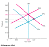
The _______ aggregate supply (LAS) curve, is vertical at potential GDP.
Long-run
Explanation
Because both the price level and the money wage rate change, the real wage rate remains constant. The real wage rate remains at the level that achieves full employment of labor. Remember, real wage rate refers to buying power – in other words, if the price of goods doubles, but your wage rate doubles as well, then your real wage rate is still the same.

A movement along the LAS curve, means that the ____ level and the money wage rate (amount of money received per worker per unit of time) are changing.
price
Explanation
Because both the price level and the money wage rate change, the real wage rate remains constant. The real wage rate remains at the level that achieves full employment of labor. Remember, real wage rate refers to buying power–in other words, if the price of goods doubles, but your wage rate doubles as well, then your real wage rate is still the same.

Short-run aggregate supply is the relationship between the quantity of real GDP supplied and the price level when the money wage rate and all other influences on _______ plans remain constant.
production
Explanation
The short-run aggregate supply (SAS) curve is upward-sloping. At a price level of 120, the quantity of real GDP supplied is $500 billion. At a price level of 130, the quantity of real GDP supplied is $600 billion, which equals potential GDP. At a price level of 140, the quantity of real GDP supplied is $700 billion, which exceeds potential GDP.

The Short-run aggregate supply (SAS) curve slopes ______.
upwards
Explanation
When the price level rises with a constant money wage rate, firms make a larger profit by producing a larger output.

A rise in both the price level and the money wage rate that maintains full employment brings a ________ along the Long-run Aggregate Supply (LAS) curve.
movement

A rise in the price level at a constant money wage rate brings a change in employment and real GDP and a movement along the _________ Aggregate Supply (SAS) curve.
Short-run

When _________ GDP increases, both LAS and SAS curves shift right.
potential
Explanation
Potential GDP changes for two basic reasons: aggregate labor hours (at full employment) increase or labor productivity increases. Labor productivity increases for three reasons: growth of the capital stock, growth of human capital, or technological change. All of these factors increase GDP and the economy will grow and prices will decrease due to the improved resource usage.

When the money wage rate _____, the SAS curve shifts left but the LAS curve remains unchanged.
rises
Explanation
The same amount will be produced but the labor input cost rises and thus the price of goods rises. The same amount of goods now cost more. This is an example of cost push inflation.

Short-run ___________ occurs when the quantity of real GDP demanded equals the quantity of real GDP supplied.
equilibrium
Explanation
Short-run equilibrium occurs at the point of intersection of the AD curve and the SAS curve. If the price level equals 130, the quantity of real GDP demanded equals the quantity of real GDP supplied. Because there is neither a surplus nor a shortage of goods and services, firms keep prices and production constant.

If the price level _______ the equilibrium price then there is a surplus of goods.
exceeds
Explanation
If the price rises above 130, the quantity of real GDP supplied exceeds the quantity of real GDP demanded. Because there is a surplus of goods and services, firms cut prices and decrease production.

If the price level falls ______ the equilibrium price then there is a shortage.
below
Explanation
If the price falls below 130, the quantity of real GDP demanded exceeds the quantity of real GDP supplied. Because there is a shortage of goods and services, firms raise prices and increase production.

A rightward shift of the ___ curve indicates economic growth.
SRS
Explanation
A leftward shift of the SAS curve indicates economic slowdown.
1) The leftward move from AS1 to AS2 results in higher prices and lower production. The rightward move from AS1 to AS3 brings decreased prices and increased production.

Long-term growth results from persistent increases in _________ GDP.
long-term
Explanation
The LAS curve (and the SAS curve) shift rightward over time. The equilibrium point is then at a higher level of production and a lower price.

_________ results from a persistent increase in aggregate demand that exceeds the increase in potential GDP.
Inflation
Explanation
The AD (Aggregate Demand) curve shifts rightward over time at a faster pace than does the LAS (Long-run Aggregate Supply) curve. The production can’t keep pace with the demand and the end result is a higher price for the same level of production. Remember, inflation is where the same amount of money is worth less.

When Aggregate Demand increases, real GDP _________.
increases
Explanation
Aggregate Demand moves from AD0 to AD1 and real GDP rises to $650 billion. This rate is above potential GDP.

When Aggregate Demand increases, the price level _________.
increases
Explanation
The price level rises to the new equilibrium point of 135.

Increased Aggregate Demand brings a(n) ________ in Short Run Aggregate Supply (SAS).
decrease
Explanation
Recall that along the SAS curve, the money wage rate is fixed but when Aggregate Demand increases, the price level increases too. This means that the real wage rate has effectively fallen (the money households earn buys them less) and the money wage rate then begins to rise. The rising real wage rate decreases short-run aggregate supply (inputs to production cost more thus supply decreases) and the SAS curve shifts leftward.

Increased Aggregate Demand brings a(n) increase in _____ level.
price
Explanation
As Aggregate demand increases, aggregate supply decreases and this pushes Real GDP back toward potential GDP - from 650 billion to 600 billion. This supply decrease is accompanied by a price level increase (145) to bring the economy back to equilibrium.

In the long run, ____ GDP is back at potential GDP.
real
Explanation
All the effects of the increase in aggregate demand have been on the price level. In the above chart: Equilibrium started at 130 then moved to 135 as Aggregate Demand shifted right. When Aggregate Supply shifted left to adjust for the increased wage rate, the equilibrium price rose again to 145.
A rise in ________ costs (labor, fuel, material, etc) will decrease SAS (Short Run Aggregate Supply).
resource
Explanation
For example, a rise in world oil prices increases costs, which means SAS shifts to the left and decreases short-run aggregate supply.

When Short Run Aggregate Supply decreases, Real GDP falls below Potential GDP and the price level _________.
increases
Explanation
In the chart: Real GDP falls to 550 billion, below potential GDP of 600 billion, and the price level rises to 140.

The following chart shows a decrease in short-run aggregate supply (from SAS0 to SAS1), with the new price level being ___.
130
Explanation
Real GDP falls to 575 and the equilibrium price is 130.

When equilibrium real GDP exceeds potential GDP, there is an __________ gap.
inflationary
Explanation
The GDP level that the market economy dictates is well beyond the current capacity, this creates high pricing and competition for product. In this example the inflationary gap is $100 billion. There is a need for $100 billion more product and service than can be provided.

When equilibrium real GDP is below potential GDP, there is a ___________ gap.
recessionary
Explanation
The GDP level that the market economy dictates is well below the current capacity, and this creates excess inventory and low pricing. The result is unemployment and decreased profit and disposable income. In this example the recessionary gap is $100 billion. There is an excess of $100 billion product and services in the economy.

The relationship between consumption expenditure and disposable income, other things remaining the same, is called the consumption ________.
function
Explanation
The consumption function plots what consumers actually spent at various levels of disposable income (DI) over a period of years. By comparing the consumption function with a 45 degree line (at each point on the line DI = Consumption), you can see the amount of money that was saved at each DI level. The point where the two lines meet is the Break even Income level.

The point on a Consumption Function where the consumption line intersects the 45 degree line is called the __________ Income level.
Break even
Explanation
This is the level at which households consume their entire incomes.

The marginal propensity to consume (MPC) is calculated as the change in __________ expenditure divided by the change in disposable income.
consumption
Explanation
Remember, MPC measures how quickly consumption changes as a result of change in income. To calculate this:

The marginal propensity to save (MPS) is calculated as the change in saving ______ by the change in disposable income.
divided
Explanation
Remember, MPS measures how much more is saved as a result of making more disposable income. For example, if you have $5,000 more to spend, how much more do you end up saving.

The slope of the consumption function equals the MPC (Marginal Propensity to _______).
Consume
