Reading 27 Risk Management Applications of Option Strategies Flashcards
Box Spreads
A box spread can also be used to exploit an arbitrage opportunity but it requires that neither the binomial nor Black–Scholes–Merton model holds, it needs no estimate of the volatility, and all of the transactions can be executed within the options market, making implementation of the strategy simpler, faster, and with lower transaction costs.
In basic terms, a box spread is a combination of a bull spread and a bear spread. Suppose we buy the call with exercise price X1 and sell the call with exercise price X2. This set of transactions is a bull spread. Then we buy the put with exercise price X2 and sell the put with exercise price X1. This is a bear spread. Intuitively, it should sound like a combination of a bull spread and a bear spread would leave the investor with a fairly neutral position, and indeed, that is the case.
(X2−X1)/(1+r)T=c1−c2+p2−p1
If some combination of the options was such that the net premium is more than the present value of the payoff, then the box spread would be overpriced.
So to summarize the box spread, we say that
- Value at expiration: VT = X2 – X1
- Profit: Π = X2 – X1 – (c1 – c2 + p2 – p1)
- Maximum profit = (same as profit)
- Maximum loss = (no loss is possible, given fair option prices)
- Breakeven: no breakeven; the transaction always earns the risk-free rate, given fair option prices
Bull Spreads
A bull spread is designed to make money when the market goes up. In this strategy we combine a long position in a call with one exercise price and a short position in a call with a higher exercise price.
To summarize the bull spread, we have:
- Value at expiration: VT = max(0,ST – X1) – max(0,ST – X2)
- Profit: Π = VT – c1 + c2
- Maximum profit = X2 – X1 – c1 + c2
- Maximum loss = c1 – c2
- Breakeven: ST* = X1 + c1 – c<span>2</span>
Bull spreads are used by investors who think the underlying price is going up.
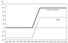
Delta Hedging an Option over Time
Two patterns become apparent:
1) The further away we move from the current price, the worse the delta-based approximation, and
2) the effects are asymmetric. A given move in one direction does not have the same effect on the option as the same move in the other direction. Specifically, for calls, the delta underestimates the effects of increases in the underlying and overestimates the effects of decreases in the underlying.
- The dealer would typically hold a position in the underlying to delta-hedge a position in the option. Trading in the underlying would not, however, always be the preferred hedge vehicle. In fact, we have stated quite strongly that trading in derivatives is often easier and more cost-effective than trading in the underlying.
- To delta hedge with options:
N1/N2=−Δc2/Δc1
* The negative sign simply means that a long position in one option will require a short position in the other. The desired quantity of Option 1 relative to the quantity of Option 2 is the ratio of the delta of Option 2 to the delta of Option 1.
Using an Interest Rate Collar with a Floating-Rate Loan
Most interest rate collars, however, are initiated by borrowers.
Butterfly Spreads
In both the bull and bear spread, we used options with two different exercise prices. There is no limit to how many different options one can use in a strategy. As an example, the butterfly spread combines a bull and bear spread. Consider three different exercise prices, X1, X2, and X3. Suppose we first construct a bull spread, buying the call with exercise price of X1 and selling the call with exercise price of X2. Recall that we could construct a bear spread using calls instead of puts. In that case, we would buy the call with the higher exercise price and sell the call with the lower exercise price. This bear spread is identical to the sale of a bull spread.
In summary, for the butterfly spread
- Value at expiration: VT = max(0,ST – X1) – 2max(0,ST – X2) + max(0,ST – X3)
- Profit: Π = VT – c1 + 2c2 – c3
- Maximum profit = X2 – X1 – c1 + 2c2 – c3
- Maximum loss = c1 – 2c2 + c3
- Breakeven: ST* = X1 + c1 – 2c2 + c3 and ST* = 2X2 – X1 – c1 + 2c2 – c3
Butterfly spread is a strategy based on the expectation of low volatility in the underlying. Of course, for a butterfly spread to be an appropriate strategy, the user must believe that the underlying will be less volatile than the market expects. If the investor buys into the strategy and the market is more volatile than expected, the strategy is likely to result in a loss. If the investor expects the market to be more volatile than he believes the market expects, the appropriate strategy could be to sell the butterfly spread. Doing so would involve selling the calls with exercise prices of X1 and X3 and buying two calls with exercise prices of X2.
Vega and Volatility Risk
The sensitivity of the option price to the volatility is called the vega and is defined as
Vega = Change in option price / Change in volatility
Dealers try to measure the vega, monitor it, and in some cases hedge it by taking on a position in another option, using that option’s vega to offset the vega on the original option. Managing vega risk, however, cannot be done independently of managing delta and gamma risk. Thus, the dealer is required to jointly monitor and manage the risk associated with the delta, gamma, and vega.
Put option: value at expiration, profit, maximum profit/loss, breakeven
Buying a put we have:
pT = max(0,X – ST)
Value at expiration = pT
Profit: Π = pT – p0
Maximum profit = X – p0
Maximum loss = p0
Breakeven: ST* = X – p0
Put–call parity
c = p + S – X/(1 + r)T
Interest rate options
The payoff of an interest rate call option is:
(Notional principal) • max (0,Underlying rate at expiration
− Exercise rate) • (Days in underlying rate/360)
If an interest rate option is used to hedge the interest paid over an m-day period, then “days in underlying” would be m.
The most important point, however, is that the rate is determined on one day, the option expiration, and payment is made m days later.
Collars
In effect, the holder of the asset gains protection below a certain level, the exercise price of the put, and pays for it by giving up gains above a certain level, the exercise price of the call. This strategy is called a collar. When the premiums offset, it is sometimes called a zero-cost collar.
In summary, for the collar:
- Value at expiration: VT = ST + max(0,X1 – ST) – max(0,ST – X2)
- Profit: Π = VT – S0
- Maximum profit = X2 – S0
- Maximum loss = S0 – X1
- Breakeven: ST* = S0
Collars are virtually the same as bull spreads.
Money Spread option strategies
A spread is a strategy in which you buy one option and sell another option that is identical to the first in all respects except either exercise price or time to expiration. If the options differ by time to expiration, the spread is called a time spread.
Gamma and the Risk of Delta
A gamma is a measure of several effects. It reflects the deviation of the exact option price change from the price change as approximated by the delta. It also measures the sensitivity of delta to a change in the underlying. In effect, it is the delta of the delta. Specifically,
Gamma = Change in delta / Change in underlying price
If a delta-hedged position were risk free, its gamma would be zero. The larger the gamma, the more the delta-hedged position deviates from being risk free.
The largest moves for gamma occur when options are trading at-the-money or near expiration, when the deltas of at-the-money options move quickly toward 1.0 or 0.0. Under these conditions, the gammas tend to be largest and delta hedges are hardest to maintain.
Formula for compounding a value at the risk-free rate for one day
Formula for compounding a value at the risk-free rate for one day is exp(rc/365)
Using an Interest Rate Floor with a Floating-Rate Loan
A combination of interest rate put options that expire on the various interest rate reset dates. This combination of puts is called a floor, and the component options are called floorlets.
Protective Put
Holding an asset and a put on the asset is a strategy known as a protective put.
Value at expiration: VT = ST + max(0,X – ST)
Profit: Π = VT – S0 – p0
Maximum profit = ∞
Maximum loss = S0 + p0 – X
Breakeven: ST* = S0 + p0
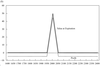
Straddle
Suppose the investor buys both a call and a put with the same exercise price on the same underlying with the same expiration. This strategy enables the investor to profit from upside or downside moves. Its cost, however, can be quite heavy. In fact, a straddle is a wager on a large movement in the underlying.
Only when the investor believes the market will be more volatile than everyone else believes would a straddle be advised.
In summary, for a straddle
- Value at expiration: VT = max(0,ST – X) + max(0,X – ST)
- Profit: Π = VT – (c0 + p0)
- Maximum profit = ∞
- Maximum loss = c0 + p0
- Breakeven: ST* = X ± (c0 + p0)
As we have noted, a straddle would tend to be used by an investor who is expecting the market to be volatile but does not have strong feelings one way or the other on the direction. An investor who leans one way or the other might consider adding a call or a put to the straddle. Adding a call to a straddle is a strategy called a strap, and adding a put to a straddle is called a strip. It is even more difficult to make a gain from these strategies than it is for a straddle, but if the hoped-for move does occur, the gains are leveraged. Another variation of the straddle is a strangle, in which the put and call have different exercise prices. This strategy creates a graph similar to a straddle but with a flat section instead of a point on the bottom.

Bear Spreads
If one uses the opposite strategy, selling a call with the lower exercise price and buying a call with the higher exercise price, the opposite results occur. The graph is completely reversed: The gain is on the downside and the loss is on the upside. This strategy is called a bear spread. The more intuitive way of executing a bear spread, however, is to use puts. Specifically, we would buy the put with the higher exercise price and sell the put with the lower exercise price.
To summarize the bear spread, we have
- Value at expiration: VT = max(0,X2 – ST) – max(0,X1 – ST)
- Profit: Π = VT – p2 + p1
- Maximum profit = X2 – X1 – p2 + p1
- Maximum loss = p2 – p1
- Breakeven: ST* = X2 – p2 + p1
The bear spread with calls involves selling the call with the lower exercise price and buying the one with the higher exercise price. Because the call with the lower exercise price will be more expensive, there will be a cash inflow at initiation of the position and hence a profit if the calls expire worthless.

Covered Call

An option strategy involving the holding of an asset and sale of a call in the asset.
Value at expiration: VT = ST – max(0,ST – X)
Profit: Π = VT – S0 + c0
Maximum profit = X – S0 + c0
Maximum loss = S0 – c0
Breakeven: ST* = S0 – c0
Finally, we should note that anecdotal evidence suggests that writers of call options make small amounts of money, but make it often. The reason for this phenomenon is generally thought to be that buyers of calls tend to be overly optimistic, but that argument is fallacious. The real reason is that the expected profits come from rare but large payoffs.
Following this line of reasoning, however, it would appear that sellers of calls can consistently take advantage of buyers of calls. That cannot possibly be the case. What happens is that buyers of calls make money less often than sellers, but when they do make money, the leverage inherent in call options amplifies their returns. Therefore, when call writers lose money, they tend to lose big, but most call writers own the underlying or are long other calls to offset the risk.