Formulas and Definitions Flashcards

1
Q

Q1=

A

0.25 (n+1)th value

OR

(n+1)/4

2
Q

Q2=

A

it’s the median

(n+1)/2

3
Q

Q3=

A

0.75 (n+1)th value

OR

3(n+1)/4

4
Q

Ecart entre 2 quartiles =

A

Interquartile range

5
Q

Median =

A

To find the Median, place the numbers in value order and find the middle.
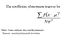
6
Q

Variance =

A

𝞼2

Average of squared differences from the mean

7
Q

Why using samples?

A

We rarely can collect data on ALL members of a population because of Time and Cost, but we still need to be able to make conclusions about the entire population.

So we use samples

8
Q

Samples guidelines and bias:

A
  • All elements in the sample must be part of the population as it’s defined
    • Bias: people under/over the age boundary
  • The sample should be representative of the population
    • Bias: collecting data on height and half of the sample plays in the NBA
  • Samples should be independent from each others
    • Bias: “Refer a friend” to the study as friends often have a lot of similarities
  • Samples are chosen randomly in many cases
    • Bias: Only choosing people from a particular background/ethnicity when the study is about a multicultural country

Sample results are ALWAYS an approximation

9
Q

Measure of Skewness

A
10
Q

Standard deviation =

A

Square root of variance

𝞼

11
Q

When should we prefer the mean or the median ?

A

The mean is mostly preferred because it uses all the data values

However, in case of extreme values, the median might be more representative

12
Q

Measures of spread VS measures of location

A
  • Sample mean and median are measures of location. They give you a ‘typical’ value of an observation.
  • Sample variance and inter-quartile range are measures of spread. They tell you how far observations tend to be from the ‘typical’ value.
  • The largest and smallest values give the range of the data, but this is not usually a robust measure of the range of values in the population (as it can vary alot among independent samples).
  • The set of five values (x(1), Q1, Q2, Q3, x(n)) is called the five point summary.
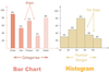
13
Q

Bar chart

VS

Histogram

VS

Box-and-whisker plot

A

Bar chart: For discrete data. Vertical bars are separate; height is proportional to frequency.

Histogram: For continuous data. Vertical bars are adjacent; if interval widths are different, the area of the rectangle is proportional to frequency.

Box-and-whisker plot: Produced with median, quartiles, max and min. The box extends from one quartile to the other, with the median marked in between.

14
Q

Symmetry:

A

Sometimes it is important to judge whether a dataset is symmetric. Look at :

  • Whether mean and median are close
  • Whether median is about midway between the quartiles
  • Whether the histogram is symmetric
15
Q

Different statistical models:

A
  • Yes/No survey (binomial)
  • Number of computer server crashes at City University per week (Poisson)
  • Returns on shares (normal)
16
Q

Standard Normal curve

A

A commonly used distribution for continuous variables is the Normal distribution illustrated below. It is symmetric. Parameters are μ, the mean, and σ the standard deviation.

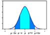
The curve in the image has a sdev of 1
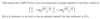
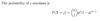
17
Q

Normal tables:

A

Z is said to have a standard normal distribution.

To calculate probabilities associated with Normal variables, use tables or computers. Normal tables usually give Φ(z) = P(Z ≤ z) only for positive numbers z. Equivalent values for negative numbers z can be found by symmetry:

18
Q

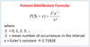
Characteristics of a Binomial Experiment:

A
  1. The process consists of a sequence of n trials
  2. Only two exclusive outcomes: success or failure
  3. Probability of success = p
  4. Probability of failure = 1-p
  5. Trials and outcomes are independent
19
Q

Binomial notations

A

X∼Binom(n,p)

20
Q

Binomial success probability formula

A

n=total population

j= success

p= probability

21
Q

Binomial coefficient calculation formula:

A

(x! on calculator)

Use nCr in calculator

22
Q

Normal approximation to Binomial:

A

When n is large, Binomial(n, p) gives roughly the same results as N (np, np(1 − p))

23
Q

Continuity correction: for X Binomial and Y Normal:

A
  • P(X > 10) = P(X 11), but
  • P(Y > 10) ≠ P(Y 11),
so we use P (Y \> 10.5) as a suitable approximation.
Similarly P(X \< 10) = P(X ≤ 9) so use P(Y \< 9.5) as an approximation.
24
Q

Random variable, Distribution and Observations:

A
  • A random variable is a numerical quantity whose value is to be determined by an experiment, but the experiment has not yet been performed.

Examples are: score on a die, height of a random student.

  • A distribution describes the values that might be observed and how likely they are. Many quantities can be assumed to have standard distributions, like Normal, Binomial.
  • After the experiment the value is known: this is an observation.

We use X, Y, Z to denote random variables, x, y, z to denote observations.

25
Q

Confidence interval

A

95% confidence interval for μ

26
Q

df=

A

Degree of freedom = sample size minus 1 = n-1

27
Q

If If σ is unknown for a confidence interval…

A

We can use S as an estimate of σ. But the distribution now changes: it is not Normal but Student’s t:

The shape of the t distribution depends on the degrees of freedom: this is n − 1 in this case. It is symmetrical about the origin.

28
Q

Confidence interval for proportions:

Normal approximation for Binomial

A

Example: in a sample of 100 people, 55 said they were opposed to the Euro. Find a CI for the population proportion.

If X is the number of people in a sample of size n who agree with a given statement, then for large n so that:

X ∼Bin(n,p) ≈ N(np,np(1−p))

  • p is unknown so the best estimator is X/n
  • The df is “infinity”

then

29
Q

Null Hypothesis =

A

H0= Null hypothesis = opposite of statement made

H1 = Alternative hypothesis = assumption being tested

30
Q

The F Test is for…

The t-test is for…

A

F: Testing whether two independent normal samples come from populations with the same variance.

t: Testing whether two independent normal samples come from populations with the same mean

The results found with the formulas should be compared to those found in the t or F tables.

tcrit lower limit is found by adding “-“ in front of the number in the table

31
Q

Use of the F Test:

A
  • The 2-sample t test can only be performed if σ12 = σ22. The F test is often used to see whether it is permissible to use the 2-sample t test. (Place the larger variance on top)
  • It has many other uses as well: see ANOVA, Linear Regression.
32
Q

When to use z or t distributions?

A

t-distribution special characteristics:

  • Sample size n≤30

and/or

  • We don’t know the variance/standard deviation
33
Q

Poisson distribution definition

A

Poisson distribution focuses on the number of discrete events or occurences over a specified interval or continuum (time, length, distance…)

34
Q

Poisson distribution formula

(ne pas apprendre?)

A
35
Q

Chi-square test formula:

A

Use the chi table to compare the results.

df= Number of categories - Number of restrictions

Number of restrictions = 1 + Number of estimated parameters

For Binomial, df= number of observation in one group - 1

36
Q

Why using ANOVA?

ANOVA Null Hypothesis:

A
  • To compare the means of more than 2 populations
  • To compare populations each containing several levels/subgroups

H0: μ1 = μ2 = µ3

37
Q

(One-way ANOVA)

Treatment?

Error?

Sum of Squares?

A

Treatment = Between = Distance of each mean from overall mean

Error = Within = Internal spread/standard deviation of each sample distribution

Sum of Squares = Sum of all squared distances from the means (SSE) / overall mean (SSTr)

38
Q

MSTr=

A

Mean Square Treatment

SSTr/dftreatment

39
Q

MSE=

A

Mean Square Error

MSE = SSE/dferror

40
Q

The p value:

A

p value < 0.05 : reject null hypothesis

p value > 0.05 : don’t reject it, (but can say “There is some evidence against H0” if 0.05 < p < 0.10)

41
Q

Assumptions for ANOVA:

A
  • Each sample comes from a population that follows a normal distribution
  • Equal Variances
  • All sample are independent and randomly selected
42
Q

Why two-way ANOVA?

A

The variations from the mean were attributed to the colums or the error with one-way ANOVA.

With two-way ANOVA we want to know which proportion of the error’s variations can be attributed to the row variations.

We want SSE to be as small as possible as we compare it to the SSC for the F-ratio

43
Q

fitted value=

A

row mean + column mean - grand mean

44
Q

residuals=

A

actual value - fitted value

45
Q

Two-way ANOVA SSE =

A

sum of squared residuals

46
Q

R2 = Coefficient of determination =

A
  • SSR / SST
  • SSTr / SST

Interpretation:

  • R2 = 0 ⇒ The dependent variable cannot be predicted using the independent one
  • R2 = 1 ⇒The dependent variable can be predicted using the independent one
  • 0 < R2 < 1 ⇒ A coefficient of determination that falls within this range measures the extent that the dependent variable is predicted by the independent variable. An R-squared of 0.20, for example, means that 20% of the dependent variable is predicted by the independent variable

A coefficient greater than 0.85 is a GOOD FIT

47
Q

“Interactions two way ANOVA:

A

An interaction means that the main effects can not be relied upon to tell the full story. When there is an interaction effect, it means the main effects do not collectively explain all of the influence of the IndependentVariables on the DependantVariable. The IVs have an interactive effect on the DV, which means the cell means must be examined for each sub-group – this is where the nature / direction of the interaction can be found.

48
Q

H0 for linear regression

A

H0= y does not depend on x

49
Q

Residuals:

A
  • Distance between “raw best-fit line” (mean of dependant variable) and the observed value. Also called Error.

SSE= Sum of Squared Errors

Raw SSE = SST

  • After conducting a regression, the SSE should be greatly diminished (becomes distance between the calculated best-fit line and the observed values). The difference SST - newSSE = SSR (regression)
50
Q

Scatter plot=

A

Coordinate plan, un repère.

The dependent variable is on the left

51
Q

Slope intercept form of a line:

A

y = α + ßx

  • x = random variable
  • ß = slope of the line (rise over run)
  • α = y-intercept (cross y-axis)
52
Q

Correlation =

A
  • r is always between -1 and 1
  • Values close to 1 show a strong positive linear relationship;
  • Values close to -1 show a strong negative linear relationship;
  • Values close to 0 indicate no linear relationship.
53
Q

Fisher’s Z:

A
  • Z is roughly N(0,1) if H0 is true.

So we reject H0 if the observed value of Z is > 1.96 or < −1.96.

54
Q

p-value

A

(1 - p(z)) * 2

55
Q

Adjusted R-squared:

A

Notice that the denominator, SST/(n−1), can alternatively be called MST.

56
Q

Multicollinearity=

A

The Independent values are potentially related to each other. There is a relationship among them.

Ideally, we don’t’ want IV to be correlated with each other. When they are, we don’t want to use them both in the multiple regression, they are redundant.

It can be tested using scatterplots and correlation