L25 - Distributed Lags

Question 1

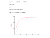
What does a scatterplot look like for a binary dependent variable?

Answer 1

• e.g. say if Y_i = {0,1}
• Then the points can only lie on the x-axis (y=0) or the line y=1 –> this makes it very hard to fit a linear equation to the scatterplot
• So instead of fitting a linear line, we fit a logistic curve with a sigmoid shape

Question 2

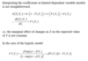
How can you interpret the coefficients in limited dependent variable models?

Answer 2

• What is the expected value of Y|X?
  
  • Well if Y can only be 0 or 1 (binary) then its expected value must be ) and 1 multiplied by the probability of occurring ( which will just leave whatever is multiplied by 1)
  • The F(X) is the conditional probability of getting Y=1
  • The first derivative gives the marginal effect of a change in X on the expected value of Y –> NOT CONSTANT
• F’(X) = β * Pr(Y=1) * Pr(Y=0)

Question 3

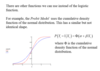
At what point do we evaluate a limited dependent variable model?

Answer 3

• at the mean of the data (use X(bar) in the calculation for the marginal effect)

Question 4

Can other functions be used to solve Limited Dependant variable models?

Answer 4

Question 5

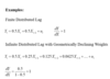
What are Distributed Lags?

Answer 5

Distributed lags are dynamic relationships in which the effects of changes in some variable X on some other variable Y are spread through time.

Distributed lags can arise for a variety of reasons including:

1. Costs of adjustment –> costly to change Y variable all at once
2. The effects of expectations –> take a while for expectations to adjust

Below depicts two ways we can account for them in a regression

Question 6

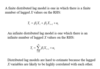
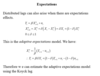
How do econometrician account for correlation between lagged X variable when using a Infinite distributed lag model?

Answer 6

• With geometrically declining weights, the future we go into the past the less of an impact its weight will have thus beta for each coefficient is halved each time
  
  • It could be said that β_i = β₀λⁱ and as long as λ < 1 (so it converges), will tend to zero –> the weights get less and less the further in the pas the lag is
  • this reduces the number of parameters we need to estimate from an infinite number of β’s to just two: β₀ and λ
• both have the same marginal effect –> the geometric sum of all the β in the infinite model = 1
  *

Question 7

How can you estimate a geometrically declining weifghts model?

Answer 7

Question 8

What is the adaptive expectation model?

Answer 8

Question 9

What is the problem with the adaptive expectations model?

Answer 9

• it is persistently and predictably wrong
  
  • it is systematic below actual inflation