Chapter 4: Normal Distribution

Question 1

The Normal Distribution

Answer 1

• The normal distribution is the most important one in all of probability and statistics.
• Many numerical populations have distributions that can be fit very closely by an appropriate normal curve.
• Examples include heights, weights, and other physical characteristics, measurement errors in scientific experiments, reaction times in psychological experiments, measurements of intelligence and aptitude, scores on various tests, and numerous economic measures and indicators.

​

Question 2

Normal Distribution definition

Answer 2

Question 3

Parameters of the Normal Distribution

Answer 3

Question 4

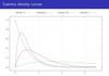
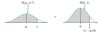
Normal Distribution Graphs with different parameters (means and variances)

Answer 4

Question 5

Normal Distribution Graphs with different parameters (means and variances) (contd.)

Answer 5

Question 6

σ and µ in Normal Distribution Graph

Answer 6

• Each density curve is symmetric about µ and bell-shaped, so the center of the bell (point of symmetry) is both the mean of the distribution and the median.
• The value of σ is the distance from µ to the inflection points of the curve (the points at which the curve changes from turning downward to turning upward).
• Large values of σ yield graphs that are quite spread out about µ, whereas small values of σ yield graphs with a high peak above m and most of the area under the graph quite close to µ.
• Thus a large σ implies that a value of X far from µ may well be observed, whereas such a value is quite unlikely when σ is small.

Question 7

Every normal curve (regardless of its mean or standard deviation) conforms to the following “rule“:​

Answer 7

• About 68% of the area under the curve falls within 1 standard deviation of the mean.
• About 95% of the area under the curve falls within 2 standard deviations of the mean.
• About 99.7% of the area under the curve falls within 3 standard deviations of the mean.
• Collectively, these points are known as the empirical rule or the 68-95-99.7 rule. Clearly, given a normal distribution, most outcomes will be within 3 standard deviations of the mean.

Question 8

The Standard Normal Distribution

Answer 8

Question 9

Parameters of a Standard Normal Distribution

Answer 9

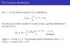
Definition
The normal distribution with parameter values µ = 0 and σ = 1 is called the standard normal distribution.
A random variable having a standard normal distribution is called a standard normal random variable and will be denoted by Z.

The pdf of Z is:

Question 10

Example 13

Answer 10

(see powerpoint slides 13-19)

Question 11

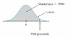
Example 14: 99th Percentile

Answer 11

• The 99th percentile of the standard normal distribution is that value on the horizontal axis such that the area under the z curve to the left of the value is .9900.
• Appendix Table A.3 , gives, for fixed z, the area under the standard normal curve to the left of z, whereas here we have the area and want the value of z.
• This is the “inverse” problem to P(Z <= z) = ?
  
  • so the table is used in an inverse fashion:
• Find in the middle of the table .9900; the row and column in which it lies identify the 99th z percentile.

Here .9901 lies at the intersection of the row marked 2.3 and column marked .03, so the 99th percentile is (approximately) z = 2.33.

Question 12

Percentiles of the Standard Normal Distribution

Answer 12

• In general, the (100p)th percentile is identified by the row and column of Appendix Table A.3 in which the entry p is found (e.g., the 67th percentile is obtained by finding .6700 in the body of the table, which gives z = .44).
• If p does not appear, the number closest to it is often used, although linear interpolation gives a more accurate answer.
• For example, to find the 95th percentile, we look for .9500 inside the table.
• Although .9500 does not appear, both .9495 and .9505 do, corresponding to z = 1.64 and 1.65, respectively.
• Since .9500 is halfway between the two probabilities that do appear, we will use 1.645 as the 95th percentile and –1.645 as the 5th percentile.

Question 13

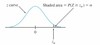
z_a Notation for z Critical Values

Answer 13

In statistical inference, we will need the values on the horizontal z-axis that capture certain small tail areas under the standard normal curve.

Notation
z_a will denote the value on the z-axis for which a (alpha) of the area under the z curve lies to the right of z_a.
(See Figure 4.19.)

For example, z_.10 captures upper-tail area .10, and z_.01 captures upper-tail area .01.

Since a (alpha) of the area under the z curve lies to the right of z_a, 1 – a of the area lies to its left. Thus z_a is the 100(1 – a)th percentile of the standard normal distribution.

By symmetry, the area under the standard normal curve to the left of –z_a is also a. The z_a’s are usually referred to as z critical values.

Question 14

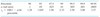
Most Useful z percentiles and z_a values

Answer 14

Question 15

Example 15

Answer 15

Question 16

Non-standard Normal Distributions

Answer 16

Question 17

Non-standard Normal Distributions (contd.)

Answer 17

Question 18

Non-standard Normal Distributions (contd. part 2)

Answer 18

The key idea of the proposition is that by standardizing, any
probability involving X can be expressed as a probability involving a standard normal rv Z, so that Appendix Table A.3 can be used.

This is illustrated in Figure 4.21.

Question 19

Example 16

• The time that it takes a driver to react to the brake lights on a decelerating vehicle is critical in helping to avoid rear-end collisions.
• The article “Fast-Rise Brake Lamp as a Collision-Prevention Device” (Ergonomics, 1993: 391–395) suggests that reaction time for an in-traffic response to a brake signal from standard brake lights can be modeled with a normal distribution having mean value 1.25 sec and standard deviation of .46 sec.

What is the probability that reaction time is between 1.00 sec and 1.75 sec?

Answer 19

Question 20

Example 16 contd.

Answer 20

Question 21

Percentiles of an Arbitrary Normal Distribution

Answer 21

Question 22

Example 18

The amount of distilled water dispensed by a certain machine is normally distributed with mean value 64 oz and standard deviation .78 oz.

What container size c will ensure that overflow occurs only .5% of the time? If X denotes the amount dispensed, the desired condition is that P(X > c) = .005, or, equivalently, that P(X <= c) = .995.

Answer 22

Thus c is the 99.5th percentile of the normal distribution with µ = 64 and σ = .78.

Question 23

Example 18 contd.

Answer 23

Question 24

The Normal Distribution and Discrete Populations

Answer 24

• The normal distribution is often used as an approximation to the distribution of values in a discrete population.
• In such situations, extra care should be taken to ensure that probabilities are computed in an accurate manner

Question 25

Normal approximation to binomial

Answer 25

Question 26

Gamma Distribution

Answer 26

Question 27

Gamma Density Curves

Answer 27

Question 28

Gamma Distribution Parameters

Answer 28

Question 29

The Chi-squared Distribution

Answer 29

Question 30

Chi-squared Densities

Answer 30

Question 31

Chi-Squared Distribution

Answer 31

• Basis for a number of procedures in statistical inference (apparent in coming lectures)
• Statistical tables for the chi-squared distribution –> Table A.7 of your text book

Question 32

Log-Normal Distribution

Answer 32

Question 33

The Weibull Distribution

Answer 33

Question 34

The Weibull Distribution (contd.)

Answer 34

Question 35

Weibull Distribution Density Curves

Answer 35

Question 36

Weibull Distribution Parameters

Answer 36

Question 37

Cdf of Weibull Distribution

Answer 37

Question 38

Example 25: Weibull Distribution

Answer 38

Question 39

Example 25: Weibull Distribution (contd.)

Answer 39

Question 40

Probability Plots Introduction

Answer 40

• An investigator will often have obtained a numerical sample x₁, x₂, …, x_n and wish to know whether it is plausible that it came from a population distribution of some particular type (e.g., from a normal distribution).
• For one thing, many formal procedures from statistical inference are based on the assumption that the population distribution is of a specified type.
• The use of such a procedure is inappropriate if the actual underlying probability distribution differs greatly from the assumed type.
• For example, the article “Toothpaste Detergents: A Potential Source of Oral Soft Tissue Damage” (Intl. J. of Dental Hygiene, 2008: 193–198) contains the following
  statement:
• “Because the sample number for each experiment (replication) was limited to three wells per treatment type, the data were assumed to be normally distributed.”
• As justification for this leap of faith, the authors wrote that “Descriptive statistics showed standard deviations that suggested a normal distribution to be highly likely.” ​Note: This argument is not very persuasive.
• Additionally, understanding the underlying distribution can sometimes give insight into the physical mechanisms involved in generating the data.
• An effective way to check a distributional assumption is to construct what is called a probability plot.

​

​

Question 41

Probability Plots

Answer 41

• The essence of such a plot is that if the distribution on which the plot is based is correct, the points in the plot should fall close to a straight line.
• If the actual distribution is quite different from the one used to construct the plot, the points will likely depart substantially from a linear pattern.

Question 42

Example 29: Probability Plots

Answer 42

• The value of a certain physical constant is known to an experimenter.
• The experimenter makes n = 10 independent measurements of this value, using a particular measurement device and records the resulting measurement errors (error = observed value – true value).
• The percentiles of the sample data appear below. The needed standard normal (z) percentiles are also displayed in the table.
• Is it plausible that the random variable measurement error has a standard normal distribution?
  • Thus the points in the probability plot are:

(–1.645, –1.91), (–1.037, –1.25),…, and (1.645, 1.56).

Question 43

Example 29: Probability Plots (contd.)

Answer 43

• Figure 4.33 shows the resulting plot. Although the points deviate a bit from the 45° line, the predominant impression is that this line fits the points very well.
• The plot suggests that the standard normal distribution is a reasonable probability model for measurement error

Question 44

Example 29: contd. pt. 2

Answer 44

• Similarly, the two largest sample observations are much smaller than the associated z percentiles.
• This plot indicates that the standard normal distribution would not be a plausible choice for the probability model that gave rise to these observed measurement errors.