DS interview questions

Question 1

50 small DT vs 1 big one

Answer 1

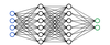
“Is a random forest a better model than a decision tree?”

• yes because a random forest is an ensemble method that takes many weak decision trees to make a strong learner.
• more accurate, more robust, and less prone to overfitting.

Question 2

Administrative datasets vs Experimental studies datasets.

Answer 2

Administrative datasets are typically

• datasets used by governments or other organizations for non-statistical reasons.
• Usually larger and more cost-efficient than experimental studies.
• Regularly updated assuming that the organization associated with the administrative dataset is active and functioning.
• May not capture all of the data that one may want and may not be in the desired format either.
• It is also prone to quality issues and missing entries.

Question 3

What is A/B testing?

Answer 3

A/B testing is a form of hypothesis testing and two-sample hypothesis testing to compare two versions, the control and variant, of a single variable. It is commonly used to improve and optimize user experience and marketing.

Question 4

Analyze a Data

Answer 4

Exploratory Data Analysis to clean, explore, and understand my data.

Compose a histogram of the duration of calls to see the underlying distribution.

Question 5

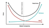
What is bias-variance trade-off?

Answer 5

Bias: Bias is an error introduced in your model due to oversimplification of the machine learning algorithm. It can lead to underfitting. When you train your model at that time model makes simplified assumptions to make the target function easier to understand.

• Low bias machine learning algorithms — Decision Trees, k-NN and SVM
• High bias machine learning algorithms — Linear Regression, Logistic Regression

Variance: Variance is error introduced in your model due to complex machine learning algorithm, your model learns noise also from the training data set and performs badly on test data set. It can lead to high sensitivity and overfitting.

Normally, as you increase the complexity of your model, you will see a reduction in error due to lower bias in the model. However, this only happens until a particular point. As you continue to make your model more complex, you end up over-fitting your model and hence your model will start suffering from high variance.

Bias-Variance trade-off: The goal of any supervised machine learning algorithm is to have low bias and low variance to achieve good prediction performance.

• The k-nearest neighbour algorithm has low bias and high variance, but the trade-off can be changed by increasing the value of k which increases the number of neighbours that contribute to the prediction and in turn increases the bias of the model.
• The support vector machine algorithm has low bias and high variance, but the trade-off can be changed by increasing the C parameter that influences the number of violations of the margin allowed in the training data which increases the bias but decreases the variance.

There is no escaping the relationship between bias and variance in machine learning. Increasing the bias will decrease the variance. Increasing the variance will decrease bias.

Question 6

How do you control for biases?

Answer 6

Two common things include randomization, where participants are assigned by chance, and random sampling, sampling in which each member has an equal probability of being chosen.

Question 7

When you sample, what bias are you inflicting?

Answer 7

• Sampling bias: a biased sample caused by non-random sampling
• Under coverage bias: sampling too few observations
• Survivorship bias: error of overlooking observations that did not make it past a form of selection process.
• Selection Bias - sample obtained is not representative of the population intended to be analysed.

Question 8

Unbalanced Binary Classification

Answer 8

• First, you want to reconsider the metrics that you’d use to evaluate your model. The accuracy of your model might not be the best metric to look at because and I’ll use an example to explain why. Let’s say 99 bank withdrawals were not fraudulent and 1 withdrawal was. If your model simply classified every instance as “not fraudulent”, it would have an accuracy of 99%! Therefore, you may want to consider using metrics like precision and recall.
• Another method to improve unbalanced binary classification is by increasing the cost of misclassifying the minority class. By increasing the penalty of such, the model should classify the minority class more accurately.
• Lastly, you can improve the balance of classes by oversampling the minority class or by undersampling the majority class.

Question 9

Boosting

Answer 9

Boosting is an ensemble method to improve a model by reducing its bias and variance, ultimately converting weak learners to strong learners.

The general idea is to train a weak learner and sequentially iterate and improve the model by learning from the previous learner.

• AdaBoost - adds weight and bias to weaker learners
• Gradient Boosting - retrained loss
• XGBoost - better/faster Gradient boosting using parallel models

Question 10

Boxplot vs Histogram

Answer 10

Boxplots and Histograms are visualizations used to show the distribution of the data

Histograms - bar charts

• show the frequency of a numerical variable’s values and are used to approximate the probability distribution of the given variable.
• It allows you to quickly understand the shape of the distribution, the variation, and potential outliers.

Boxplots

• you can gather other information like the quartiles, the range, and outliers.
• useful when you want to compare multiple charts at the same time because they take up less space than histograms.

Question 11

Central Limit Theorem

Answer 11

CLT - sampling distribution of the sample mean approaches a normal distribution as the sample size gets larger no matter what the shape of the population distribution.

The central limit theorem is important because it is used in hypothesis testing and also to calculate confidence intervals.

Question 12

What is Cluster Sampling?

Answer 12

Cluster sampling is a technique used when it becomes difficult to study the target population spread across a wide area and simple random sampling cannot be applied. Cluster Sample is a probability sample where each sampling unit is a collection or cluster of elements.

For eg., A researcher wants to survey the academic performance of high school students in Japan. He can divide the entire population of Japan into different clusters (cities). Then the researcher selects a number of clusters depending on his research through simple or systematic random sampling.

Question 13

Collinearity / Multi-collinearity

Answer 13

Multicollinearity exists when an independent variable is highly correlated with another independent variable in a multiple regression equation. This can be problematic because it undermines the statistical significance of an independent variable.

You could use the Variance Inflation Factors (VIF) to determine if there is any multicollinearity between independent variables — a standard benchmark is that if the VIF is greater than 5 then multicollinearity exists.

Question 14

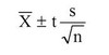
In a study of emergency room waiting times, investigators consider a new and the standard triage systems. To test the systems, administrators selected 20 nights and randomly assigned the new triage system to be used on 10 nights and the standard system on the remaining 10 nights. They calculated the nightly median waiting time (MWT) to see a physician. The average MWT for the new system was 3 hours with a variance of 0.60 while the average MWT for the old system was 5 hours with a variance of 0.68. Consider the 95% confidence interval estimate for the differences of the mean MWT associated with the new system. Assume a constant variance. What is the interval? Subtract in this order (New System — Old System).

Answer 14

https://miro.medium.com/max/776/0*QpSg349Ozhe-etIQ.png

Confidence Interval = mean +/- t-score * standard error (see above)

mean = new mean — old mean = 3–5 = -2

t-score = 2.101 given df=18 (20–2) and confidence interval of 95%

standard error = sqrt((0.⁶²*9+0.⁶⁸²*9)/(10+10–2)) * sqrt(1/10+1/10)
standard error = 0.352

confidence interval = [-2.75, -1.25]

Question 15

To further test the hospital triage system, administrators selected 200 nights and randomly assigned a new triage system to be used on 100 nights and a standard system on the remaining 100 nights. They calculated the nightly median waiting time (MWT) to see a physician. The average MWT for the new system was 4 hours with a standard deviation of 0.5 hours while the average MWT for the old system was 6 hours with a standard deviation of 2 hours. Consider the hypothesis of a decrease in the mean MWT associated with the new treatment. What does the 95% independent group confidence interval with unequal variances suggest vis a vis this hypothesis? (Because there’s so many observations per group, just use the Z quantile instead of the T.)

Answer 15

Assuming we subtract in this order (New System — Old System):

confidence interval formula for two independent samples

mean = new mean — old mean = 4–6 = -2

z-score = 1.96 confidence interval of 95%

st. error = sqrt((0.⁵²*99+²²*99)/(100+100–2)) * sqrt(1/100+1/100)
standard error = 0.205061
lower bound = -2–1.96*0.205061 = -2.40192
upper bound = -2+1.96*0.205061 = -1.59808

confidence interval = [-2.40192, -1.59808]

Question 16

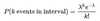
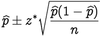
You are running for office and your pollster polled hundred people. Sixty of them claimed they will vote for you. Can you relax?

Answer 16

• Assume that there’s only you and one other opponent.
• Also, assume that we want a 95% confidence interval. This gives us a z-score of 1.96.

p-hat = 60/100 = 0.6
z* = 1.96
n = 100
This gives us a confidence interval of [50.4,69.6]. Therefore, given a confidence interval of 95%, if you are okay with the worst scenario of tying then you can relax. Otherwise, you cannot relax until you got 61 out of 100 to claim yes.

Question 17

In a population of interest, a sample of 9 men yielded a sample average brain volume of 1,100cc and a standard deviation of 30cc. What is a 95% Student’s T confidence interval for the mean brain volume in this new population?

Answer 17

Given a confidence level of 95% and degrees of freedom equal to 8, the t-score = 2.306

Confidence interval = 1100 +/- 2.306*(30/3)
Confidence interval = [1076.94, 1123.06]

Question 18

A diet pill is given to 9 subjects over six weeks. The average difference in weight (follow up — baseline) is -2 pounds. What would the standard deviation of the difference in weight have to be for the upper endpoint of the 95% T confidence interval to touch 0?

Answer 18

Upper bound = mean + t-score*(standard deviation/sqrt(sample size))
0 = -2 + 2.306*(s/3)
2 = 2.306 * s / 3
s = 2.601903
Therefore the standard deviation would have to be at least approximately 2.60 for the upper bound of the 95% T confidence interval to touch 0.

Question 19

What is the difference between Point Estimates and Confidence Interval?

Answer 19

Point Estimation gives us a particular value as an estimate of a population parameter. Method of Moments and Maximum Likelihood estimator methods are used to derive Point Estimators for population parameters.

A confidence interval gives us a range of values which is likely to contain the population parameter. The confidence interval is generally preferred, as it tells us how likely this interval is to contain the population parameter. This likeliness or probability is called Confidence Level or Confidence coefficient and represented by 1 — alpha, where alpha is the level of significance.

Question 20

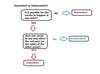
What are confounding variables?

Answer 20

A confounding variable, or a confounder, is

• a variable that influences both the dependent variable and the independent variable, causing a spurious association,
• a mathematical relationship in which two or more variables are associated but not causally related.

Question 21

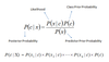
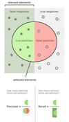
What is a confusion matrix?

Answer 21

The confusion matrix is a 2X2 table that contains 4 outputs provided by the binary classifier. Various measures, such as error-rate, accuracy, specificity, sensitivity, precision and recall are derived from it.

A binary classifier predicts all data instances of a test data set as either positive or negative. This produces four outcomes:

1. True-positive(TP) — Correct positive prediction
2. False-positive(FP) — Incorrect positive prediction
3. True-negative(TN) — Correct negative prediction
4. False-negative(FN) — Incorrect negative prediction

Basic measures derived from the confusion matrix

• Error Rate = (FP+FN)/(P+N)
• Accuracy = (TP+TN)/(P+N)
• Sensitivity(Recall or True positive rate) = TP/P = TP/(TP+FN)
• Specificity(True negative rate) = TN/N = TN/(TN+FP)
• Precision(Positive predicted value) = TP/(TP+FP)
• F-Score(Harmonic mean of precision and recall) = (1+b)(PREC.REC)/(b²PREC+REC) where b is commonly 0.5, 1, 2.
  F1-Score = (2 * Precision * Recall) / (Precision + Recall)

Question 22

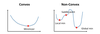
Convex vs Non-Convex cost function

Answer 22

A convex function is one where a line drawn between any two points on the graph lies on or above the graph. It has one minimum.

A non-convex function is one where a line drawn between any two points on the graph may intersect other points on the graph. It characterized as “wavy”.

When a cost function is non-convex, it means that there’s a likelihood that the function may find local minima instead of the global minimum, which is typically undesired in machine learning models from an optimization perspective.

Question 23

What is correlation and covariance in statistics?

Answer 23

Both Correlation and Covariance establish the relationship and also measure the dependency between two random variables.

Correlation: Correlation is considered or described as the best technique for measuring and also for estimating the quantitative relationship between two variables. Correlation measures how strongly two variables are related.

Covariance: In covariance two items vary together and it’s a measure that indicates the extent to which two random variables change in cycle. It is a statistical term; it explains the systematic relation between a pair of random variables, wherein changes in one variable reciprocal by a corresponding change in another variable.

Question 24

Cross-Validation

Answer 24

Cross-validation is essentially a technique used to assess how well a model performs on a new independent dataset. The simplest example of cross-validation is when you split your data into two groups: training data and testing data, where you use the training data to build the model and the testing data to test the model.

The goal of cross-validation is to limit problems like overfitting and get an insight on how the model will generalize to an independent data set.

Question 25

How does data cleaning plays a vital role in the analysis?

Answer 25

Data cleaning can help in analysis because: * Cleaning data from multiple sources **helps to transform it into a format that data analysts or data scientists can work with.** * Data Cleaning **helps to increase the accuracy of the model** in machine learning. * It is a cumbersome process because as the number of data sources increases, the time taken to clean the data increases exponentially due to the number of sources and the volume of data generated by these sources. * It might take up to 80% of the time for just cleaning data making it a critical part of the analysis task.

Question 26

Data Wrangling / Cleaning

Answer 26

* **Data profiling**: Almost everyone starts off by getting an understanding of their dataset. More specifically, you can look at the shape of the dataset with .shape and a description of your numerical variables with .describe(). * **Data visualizations**: Sometimes, it’s useful to visualize your data with histograms, boxplots, and scatterplots to better understand the relationships between variables and also to identify potential outliers. * **Syntax error**: This includes making sure there’s no white space, making sure letter casing is consistent, and checking for typos. You can check for typos by using .unique() or by using bar graphs. * **Standardization** or **normalization**: Depending on the dataset your working with and the machine learning method you decide to use, it may be useful to standardize or normalize your data so that different scales of different variables don’t negatively impact the performance of your model. * **Handling null values**: There are a number of ways to handle null values including deleting rows with null values altogether, replacing null values with the mean/median/mode, replacing null values with a new category (eg. unknown), predicting the values, or using machine learning models that can deal with null values. Read more here. * **Other** things include: removing irrelevant data, removing duplicates, and type conversion.

Question 27

Decision Tree

Answer 27

**Decision trees** * popular model, used in operations research, strategic planning, and machine learning. * Each square above is called a node, and the more nodes you have, the more accurate your decision tree will be (generally). The last nodes of the decision tree, where a decision is made, are called the leaves of the tree. * Decision trees are intuitive and easy to build but fall short when it comes to accuracy.

Question 28

Dimension Reduction

Answer 28

Dimensionality reduction is the **process of reducing the number of features in a dataset**. This is *important mainly in the case when you want to reduce variance in your model (overfitting)*. Four advantages of dimensionality reduction: * It **reduces the time and storage space required** * **Removal of multi-collinearity** improves the interpretation of the parameters of the machine learning model * It becomes **easier to visualize the data** when reduced to very low dimensions such as 2D or 3D * It **avoids the curse of dimensionality**

Question 29

Dimensionality Reduction before fitting

Answer 29

When the **number of features is greater than the number of observations**, then performing dimensionality reduction will generally improve the SVM.

Question 30

What are Eigenvectors and Eigenvalues?

Answer 30

**Eigenvectors** are used for understanding linear transformations. In data analysis, we usually calculate the eigenvectors for a correlation or covariance matrix. Eigenvectors are the **directions along which a particular linear transformation acts by flipping, compressing or stretching.** **Eigenvalue** can be referred to as the strength of the transformation in the direction of eigenvector or the factor by which the compression occurs.

Question 31

**Experimental** data vs **Observational** data

Answer 31

**Observational data** comes from observational studies which are when you *observe certain variables and try to determine if there is any correlation.* **Experimental data** comes from experimental studies which are when you *control certain variables and hold them constant to determine if there is any causality.* * An example of experimental design is the following: split a group up into two. The control group lives their lives normally. The test group is told to drink a glass of wine every night for 30 days. Then research can be conducted to see how wine affects sleep.

Question 32

**False Positive** vs **False Negative**

Answer 32

**False positive** is an incorrect identification of the presence of a condition when it’s absent. * predict positive when actual value is negative * spam dectection **False negative** is an incorrect identification of the absence of a condition when it’s actually present. * predict negative when actual value is positive * screening for cancer. This is a subjective argument, but false positives can be worse than false negatives from a psychological point of view. For example, a false positive for winning the lottery could be a worse outcome than a false negative because people normally don’t expect to win the lottery anyways.

Question 33

Suppose that diastolic blood pressures (DBPs) for men aged 35–44 are normally distributed with a mean of 80 (mm Hg) and a standard deviation of 10. About what is the probability that a random 35–44 year old has a DBP less than 70?

Answer 33

Since 70 is one standard deviation below the mean, take the area of the Gaussian distribution to the left of one standard deviation. = 2.3 + 13.6 = 15.9%

Question 34

How do you prove that males are on average taller than females by knowing just gender height?

Answer 34

* **Null hypothesis**: males and females are the same height on average * **Alternative hypothesis**: the average height of males is greater than the average height of females. * **Collect random sample** of heights of males and females and * Use a **t-test** to determine if you reject the null or not.

Question 35

Kernel

Answer 35

* A **kernel** is a way of computing the **dot product of two vectors 𝐱x and 𝐲y** in some (possibly very high dimensional) feature space, which is why kernel functions are sometimes called “*generalized dot product*” [2] * The kernel *trick is a method of using a linear classifier to solve a non-linear problem by transforming linearly inseparable data to linearly separable ones in a higher dimension.*

Question 36

What is the **Law of Large Numbers**?

Answer 36

The Law of Large Numbers is a theory that states that as the number of trials increases, the average of the result will become closer to the expected value. It says that the sample means, the sample variance and the sample standard deviation converge to what they are trying to estimate. Eg. flipping heads from fair coin 100,000 times should be closer to 0.5 than 100 times.

Question 37

What is: lift, KPI, robustness, model fitting, design of experiments, 80/20 rule?

Answer 37

**Lift**: lift is a measure of the performance of a targeting model measured against a random choice targeting model; in other words, lift tells you how much better your model is at predicting things than if you had no model. **KPI**: stands for Key Performance Indicator, which is a measurable metric used to determine how well a company is achieving its business objectives. Eg. error rate. **Robustness**: generally robustness refers to a system’s ability to handle variability and remain effective. **Model fitting**: refers to how well a model fits a set of observations. **Design of experiments**: also known as DOE, it is the design of any task that aims to describe and explain the variation of information under conditions that are hypothesized to reflect the variable. [4] In essence, an experiment aims to predict an outcome based on a change in one or more inputs (independent variables). **80/20 rule**: also known as the Pareto principle; states that 80% of the effects come from 20% of the causes. Eg. 80% of sales come from 20% of customers.

Question 38

# 20 Linear Model

Answer 38

Linear Model assumptions: * **Linear relationship** - relationship between the independent and dependent variables to be linear. The linearity assumption can best be tested with scatter plots, and a regression line. * **Multivariate normality** - data (all variables) normally distributed, bell curve test with Histogram plot * **No or little multicollinearity** - Multicollinearity occurs when the independent variables are too highly correlated with each other. Simplest way to address the problem is to remove independent variables with high VIF values. ​Multicollinearity may be tested with three central criteria: 1. **Correlation matrix** - Pearson’s Bivariate Correlation 2. **Tolerance** - measures the influence of one independent variable on all other independent variables; the tolerance is calculated with an initial linear regression analysis. 3. **Variance Inflation Factor (VIF)** - With VIF \> 5 there is an indication that multicollinearity may be present; with VIF \> 10 there is certainly multicollinearity among the variables. * **No auto-correlation** - Autocorrelation occurs when the residuals are not independent from each other. Durbin-Watson test for auto-correlation. * **Homoscedasticity** - The scatter plot is good way to check whether the data are homoscedastic (*meaning the residuals are equal across the regression line*).

Question 39

# 17 Linear Regression assumptions

Answer 39

Same as Linear Model assumptions: * The sample data used to fit the model is **representative of the population** * The relationship between X and the mean of Y is **linear** * The variance of the residual is the same for any value of X (**homoscedasticity**) * Observations are **independent of each other** * For any value of X, Y is **normally distributed**. * Extreme violations* of these assumptions will make the **results redundant**. * Small violations* of these assumptions will result in a **greater bias or variance of the estimate.**

Question 40

What is the difference between “long” and “wide” format data?

Answer 40

* In the wide-format, a subject’s repeated responses will be in a single row, and each response is in a separate column. * In the long-format, each row is a one-time point per subject. You can recognize data in wide format by the fact that columns generally represent groups.

Question 41

Long-tailed Distribution

Answer 41

A long-tailed distribution is a type of heavy-tailed distribution that has a tail (or tails) that drop off gradually and asymptotically. It’s important to be mindful of long-tailed distributions in classification and regression problems because the least frequently occurring values make up the majority of the population. This can ultimately change the way that you deal with outliers, and it also conflicts with some machine learning techniques with the assumption that the data is normally distributed. 3 practical examples include the power law, the Pareto principle (more commonly known as the 80–20 rule), and product sales (i.e. best selling products vs others).

Question 42

Markov Chains

Answer 42

A Markov chain is a mathematical system that experiences transitions from one state to another according to certain probabilistic rules. The defining characteristic of a Markov chain is that no matter how the process arrived at its present state, the possible future states are fixed. In other words, the probability of transitioning to any particular state is dependent solely on the current state and time elapsed.

Question 43

Mean Imputation

Answer 43

**Mean imputation** is the practice of replacing null values in a data set with the mean of the data. * Mean imputation is generally bad practice because **it doesn’t take into account feature correlation**. For example, imagine we have a table showing age and fitness score and imagine that an eighty-year-old has a missing fitness score. If we took the average fitness score from an age range of 15 to 80, then the eighty-year-old will appear to have a much higher fitness score that he actually should. * Second, mean imputation **reduces the variance of the data and increases bias in our data**. This leads to a less accurate model and a narrower confidence interval due to a smaller variance.

Question 44

Give an example where the **Median** is a better measure than the **Mean**

Answer 44

When there are a number of outliers that positively or negatively **skew** the data.

Question 45

How to define/select **metrics**

Answer 45

The metric(s) chosen to evaluate a machine learning model depends on various factors: * Is it a **regression or classification** task? * What is the business objective? Eg. **precision vs recall** * What is the **distribution of the target variable**? There are a number of metrics that can be used, including adjusted r-squared, MAE, MSE, accuracy, recall, precision, f1 score, and the list goes on.

Question 46

Missing Data

Answer 46

There are several ways to handle missing data: * Delete rows with missing data * Mean/Median/Mode imputation * Assigning a unique value * Predicting the missing values * Using an algorithm which supports missing values, like random forests

Question 47

MSE

Answer 47

**Mean Squared Error** (MSE) - * gives a relatively high weight to large errors * put too much emphasis on large deviations. * A more robust alternative is **MAE** (mean absolute deviation).

Question 48

Naive Bayes

Answer 48

One major drawback of Naive Bayes is that it holds a strong **assumption in that the features are assumed to be uncorrelated** with one another, which typically is never the case. One way to **improve such an algorithm that uses Naive Bayes is by decorrelating the features** so that the assumption holds true. Pros: * Easy and fast. * works for multi class prediction * performs great when independence assumption holds true * also performs well with bell curve assumption Cons: * Category in test data not mentioned in train data will result in 0 probalility. * almost impossible to find data with no correlation

Question 49

Neural Network

Answer 49

* A **neural network** is a **multi-layered** model inspired by the human brain. Like the neurons in our brain, the circles above represent a node. * The blue circles represent the **input layer**, the black circles represent the **hidden layers**, and the green circles represent the **output layer**. * Each node in the hidden layers represents a function that the inputs go through, ultimately leading to an output in the green circles. The formal term for these functions is called the sigmoid **activation function**.

Question 50

NLP

Answer 50

**Natural Language Processing** * It is a branch of artificial intelligence that gives machines the ability to **read and understand human languages**.

Question 51

Give examples of data that does not have a Gaussian distribution, nor log-normal.

Answer 51

* Any type of **categorical data** won’t have a gaussian distribution or lognormal distribution. * **Exponential distributions** — eg. the amount of time that a car battery lasts or the amount of time until an earthquake occurs.

Question 52

What do you understand by the term Normal Distribution?

Answer 52

Data is distributed around a central value without any bias to the left or right and reaches normal distribution in the form of a bell-shaped curve. The random variables are distributed in the form of a symmetrical, bell-shaped curve. Properties of Normal Distribution are as follows; * Unimodal -one mode * Symmetrical -left and right halves are mirror images * Bell-shaped -maximum height (mode) at the mean * Mean, Mode, and Median are all located in the center * Asymptotic

Question 53

Outlier

Answer 53

**Outlier**: * Data point that differs significantly from other observations. * hey can be bad from a machine learning perspective because they can worsen the accuracy of a model. * it’s important to remove them from the dataset. * identify outliers: * **Z-score/standard deviations**: if we know that 99.7% of data in a data set lie within three standard deviations, then we can calculate the size of one standard deviation, multiply it by 3, and identify the data points that are outside of this range. Likewise, we can calculate the z-score of a given point, and if it’s equal to +/- 3, then it’s an outlier. (data needs to be not small and normally distributed) * **Interquartile Range (IQR)**: IQR, the concept used to build boxplots, can also be used to identify outliers. * Other methods include **DBScan clustering**, **Isolation Forests**, and **Robust Random Cut Forests**. **Inlier**: * Data observation that lies within the rest of the dataset and is unusual or an error. * it is typically harder to identify than an outlier and requires external data to identify them. * Should you identify any inliers, you can simply remove them from the dataset to address them.

Question 54

What are the differences between over-fitting and under-fitting?

Answer 54

In **overfitting**, a statistical model *describes random error or noise instead of the underlying relationship*. Overfitting **occurs when a model is excessively complex, such as having too many parameters relative to the number of observations**. A model that has been overfitted, has *poor predictive performance*, as it overreacts to minor fluctuations in the training data. **Underfitting** occurs when a statistical model or machine learning **algorithm cannot capture the underlying trend of the data**. Underfitting would occur, for example, **when fitting a linear model to non-linear data**. Such a model too would have **poor predictive performance**.

Question 55

Overfitting

Answer 55

**Overfitting** is an error where the **model ‘fits’ the data too well**, resulting in a model with **high variance and low bias**. As a consequence, an overfit model will **inaccurately predict new data points** even though it has a high accuracy on the training data.

Question 56

How to combat Overfitting and Underfitting?

Answer 56

To combat overfitting and underfitting, you can **resample the data** to estimate the model accuracy (**k-fold cross-validation**) and by having a **validation dataset** to evaluate the model.

Question 57

P(A|B)

Answer 57

Bayes's formula: p(A|B) = (p(B|A)\*p(A))/p(A) = p(A and B)/p(A)

Question 58

What is p-value?

Answer 58

When you perform a *hypothesis test* in statistics, a **p-value can help you determine the strength of your results**. p-value is a number between 0 and 1. Based on the value it will denote the strength of the results. The claim which is on trial is called the Null Hypothesis. Low p-value (≤ 0.05) indicates strength against the null hypothesis which means we can reject the null Hypothesis. High p-value (≥ 0.05) indicates strength for the null hypothesis which means we can accept the null Hypothesis p-value of 0.05 indicates the Hypothesis could go either way. To put it in another way, * **High P values**: your data are likely with a true null. * **Low P values**: your data are unlikely with a true null.

Question 59

Infection rates at a hospital above a 1 infection per 100 person-days at risk are considered high. A hospital had 10 infections over the last 1787 person-days at risk. Give the p-value of the correct one-sided test of whether the hospital is below the standard.

Answer 59

Since we looking at the number of events (# of infections) occurring within a given timeframe, this is a **Poisson distribution** question. The probability of observing k events in an interval * *Null** (H0): 1 infection per person-days * *Alternative** (H1): \>1 infection per person-days k (actual) = 10 infections lambda (theoretical) = (1/100)\*1787 p = 0.032372 or 3.2372% *calculated using .poisson() in excel or ppois in R* Since p-value \< alpha (assuming 5% level of significance), we reject the null and conclude that the hospital is below the standard.

Question 60

PCA

Answer 60

**Principal Component Analysis,** PCA, involves project **higher dimensional data (eg. 3 dimensions) to a smaller space (eg. 2 dimensions**). This results in a lower dimension of data, (2 dimensions instead of 3 dimensions) while keeping all original variables in the model. PCA is commonly *used for compression purposes, to reduce required memory and to speed up the algorithm, as well as for visualization purposes, making it easier to summarize data.*

Question 61

Geiger counter records 100 radioactive decays in 5 minutes. Find an approximate 95% interval for the number of decays per hour.

Answer 61

* Since this is a Poisson distribution question, mean = lambda = variance, which also means that standard deviation = square root of the mean * a 95% confidence interval implies a z score of 1.96 * one standard deviation = 10 Therefore the confidence interval = 100 +/- 19.6 = [964.8, 1435.2]

Question 62

The homicide rate in Scotland fell last year to 99 from 115 the year before. Is this reported change really noteworthy?

Answer 62

* Since this is a Poisson distribution question, mean = lambda = variance, which also means that standard deviation = square root of the mean * a 95% confidence interval implies a z score of 1.96 * one standard deviation = sqrt(115) = 10.724 Therefore the confidence interval = 115+/- 21.45 = [93.55, 136.45]. Since 99 is within this confidence interval, we can assume that this change is not very noteworthy.

Question 63

**Precision** and **Recall**

Answer 63

**Recall** - proportion of actual positives was identified correctly * Recall = TP/(TP+FN) **Precision** - proportion of positive identifications was actually correct * Precision = TP/(TP+FP)

Question 64

An HIV test has a sensitivity of 99.7% and a specificity of 98.5%. A subject from a population of prevalence 0.1% receives a positive test result. What is the precision of the test (i.e the probability he is HIV positive)?

Answer 64

``` Precision = Positive Predictive Value = PV PV = (0.001\*0.997)/[(0.001\*0.997)+((1–0.001)\*(1–0.985))] PV = 0.0624 or 6.24% ```

Question 65

A certain couple tells you that they have two children, at least one of which is a girl. What is the probability that they have two girls?

Answer 65

3 possibilities of BG, GB & BB, we have to find the probability of the case with two girls. Thus, P(Having two girls given one girl) = 1 / 3

Question 66

How can you tell if a given coin is biased?

Answer 66

Perform a hypothesis test: 1. The null hypothesis is that the coin is not biased and the probability of flipping heads should equal 50% (p=0.5). The alternative hypothesis is that the coin is biased and p != 0.5. 2. Flip the coin 500 times. 3. Calculate Z-score (if the sample is less than 30, you would calculate the t-statistics). 4. Compare against alpha (two-tailed test so 0.05/2 = 0.025). 5. If p-value \> alpha, the null is not rejected and the coin is not biased. If p-value \< alpha, the null is rejected and the coin is biased.

Question 67

You are about to get on a plane to London, you want to know whether you have to bring an umbrella or not. You call three of your random friends and ask each one of them if it’s raining. The probability that your friend is telling the truth is 2/3 and the probability that they are playing a prank on you by lying is 1/3. If all 3 of them tell that it is raining, then what is the probability that it is actually raining in London.

Answer 67

You can tell that this question is related to Bayesian theory because of the last statement which essentially follows the structure, “What is the probability A is true given B is true?” Therefore we need to know the probability of it raining in London on a given day. Let’s assume it’s 25%. P(A) = probability of it raining = 25% P(B) = probability of all 3 friends say that it’s raining P(A|B) probability that it’s raining given they’re telling that it is raining P(B|A) probability that all 3 friends say that it’s raining given it’s raining = (2/3)³ = 8/27 Step 1: Solve for P(B) P(A|B) = P(B|A) \* P(A) / P(B), can be rewritten as P(B) = P(B|A) \* P(A) + P(B|not A) \* P(not A) P(B) = (2/3)³ \* 0.25 + (1/3)³ \* 0.75 = 0.25\*8/27 + 0.75\*1/27 Step 2: Solve for P(A|B) P(A|B) = 0.25 \* (8/27) / ( 0.25\*8/27 + 0.75\*1/27) P(A|B) = 8 / (8 + 3) = 8/11 Therefore, if all three friends say that it’s raining, then there’s an 8/11 chance that it’s actually raining.

Question 68

You roll a biased coin (p(head)=0.8) five times. What’s the probability of getting three or more heads?

Answer 68

General Binomial Probability formula: ``` p = 0.8 n = 5 k = 3,4,5 ``` P(3 or more heads) = P(3 heads) + P(4 heads) + P(5 heads) = 0.94 or 94%

Question 69

You are given 40 cards with four different colors- 10 Green cards, 10 Red Cards, 10 Blue cards, and 10 Yellow cards. The cards of each color are numbered from one to ten. Two cards are picked at random. Find out the probability that the cards picked are not of the same number and same color.

Answer 69

Since these events are not independent, we can use the rule: P(A and B) = P(A) \* P(B|A) ,which is also equal to P(not A and not B) = P(not A) \* P(not B | not A) For example: P(not 4 and not yellow) = P(not 4) \* P(not yellow | not 4) P(not 4 and not yellow) = (36/39) \* (27/36) P(not 4 and not yellow) = 0.692 Therefore, the probability that the cards picked are not the same number and the same color is 69.2%.

Question 70

You are at a Casino and have two dices to play with. You win $10 every time you roll a 5. If you play till you win and then stop, what is the expected payout?

Answer 70

* Let’s assume that it costs $5 every time you want to play. * There are 36 possible combinations with two dice. * Of the 36 combinations, there are 4 combinations that result in rolling a five (see blue). This means that there is a 4/36 or 1/9 chance of rolling a 5. * A 1/9 chance of winning means you’ll lose eight times and win once (theoretically). * Therefore, your expected payout is equal to $10.00 \* 1 — $5.00 \* 9= -$35.00.

Question 71

How can you generate a random number between 1 – 7 with only a die?

Answer 71

(note: I don't agree, need to do this myself) * Any die has six sides from 1-6. There is no way to get seven equal outcomes from a single rolling of a die. If we roll the die twice and consider the event of two rolls, we now have 36 different outcomes. * To get our 7 equal outcomes we have to reduce this 36 to a number divisible by 7. We can thus consider only 35 outcomes and exclude the other one. * A simple scenario can be to exclude the combination (6,6), i.e., to roll the die again if 6 appears twice. * All the remaining combinations from (1,1) till (6,5) can be divided into 7 parts of 5 each. This way all the seven sets of outcomes are equally likely.

Question 72

A box has 12 red cards and 12 black cards. Another box has 24 red cards and 24 black cards. You want to draw two cards at random from one of the two boxes, one card at a time. Which box has a higher probability of getting cards of the same color and why?

Answer 72

The box with 24 red cards and 24 black cards has a higher probability of getting two cards of the same color. Let’s walk through each step. Let’s say the first card you draw from each deck is a red Ace. This means that in the deck with 12 reds and 12 blacks, there’s now 11 reds and 12 blacks. Therefore your odds of drawing another red are equal to 11/(11+12) or 11/23. In the deck with 24 reds and 24 blacks, there would then be 23 reds and 24 blacks. Therefore your odds of drawing another red are equal to 23/(23+24) or 23/47. Since 23/47 \> 11/23, the second deck with more cards has a higher probability of getting the same two cards

Question 73

A jar has 1000 coins, of which 999 are fair and 1 is double headed. Pick a coin at random, and toss it 10 times. Given that you see 10 heads, what is the probability that the next toss of that coin is also a head?

Answer 73

There are two ways of choosing the coin. One is to pick a fair coin and the other is to pick the one with two heads. Probability of selecting fair coin = 999/1000 = 0.999 Probability of selecting unfair coin = 1/1000 = 0.001 Selecting 10 heads in a row = Selecting fair coin \* Getting 10 heads + Selecting an unfair coin P (A) = 0.999 \* (1/2)^5 = 0.999 \* (1/1024) = 0.000976 P (B) = 0.001 \* 1 = 0.001 P( A / A + B ) = 0.000976 / (0.000976 + 0.001) = 0.4939 P( B / A + B ) = 0.001 / 0.001976 = 0.5061 Probability of selecting another head = P(A/A+B) \* 0.5 + P(B/A+B) \* 1 = 0.4939 \* 0.5 + 0.5061 = 0.7531

Question 74

Consider influenza epidemics for two-parent heterosexual families. Suppose that the probability is 17% that at least one of the parents has contracted the disease. The probability that the father has contracted influenza is 12% while the probability that both the mother and father have contracted the disease is 6%. What is the probability that the mother has contracted influenza?

Answer 74

Using the General Addition Rule in probability: P(mother or father) = P(mother) + P(father) — P(mother and father) P(mother) = P(mother or father) + P(mother and father) — P(father) P(mother) = 0.17 + 0.06–0.12 P(mother) = 0.11

Question 75

In any 15-minute interval, there is a 20% probability that you will see at least one shooting star. What is the proba­bility that you see at least one shooting star in the period of an hour?

Answer 75

(billy's note: not sure i agree, need to do this myself) Probability of not seeing any shooting star in 15 minutes is = 1 – P( Seeing one shooting star ) = 1 – 0.2 = 0.8 Probability of not seeing any shooting star in the period of one hour = (0.8) ^ 4 = 0.4096 Probability of seeing at least one shooting star in the one hour = 1 – P( Not seeing any star ) = 1 – 0.4096 = 0.5904

Question 76

Given two fair dices, what is the probability of getting scores that sum to 4? to 8?

Answer 76

* There are 4 combinations of rolling a 4 (1+3, 3+1, 2+2): P(rolling a 4) = 3/36 = 1/12 * There are combinations of rolling an 8 (2+6, 6+2, 3+5, 5+3, 4+4): P(rolling an 8) = 5/36

Question 77

Make an unfair coin fair

Answer 77

Since a coin flip is a binary outcome, you can make an unfair coin fair by flipping it twice. If you flip it twice, there are two outcomes that you can bet on: heads followed by tails or tails followed by heads. *P(heads) \* P(tails) = P(tails) \* P(heads)* This makes sense since each coin toss is an independent event. This means that if you get heads → heads or tails → tails, you would need to reflip the coin.

Question 78

Probability Fundamentals

Answer 78

Eight rules of probability: 1. For any event A, 0 ≤ P(A) ≤ 1; in other words, the **probability** of an event can **range from 0 to 1**. 2. The **sum of the probabilities** of all possible outcomes always **equals 1.** 3. **P(not A) = 1 — P(A)**; This rule explains the relationship between the probability of an event and its complement event. A complement event is one that includes all possible outcomes that aren’t in A. 4. If **A and B are disjoint** events (mutually exclusive), then **P(A or B) = P(A) + P(B)**; this is called the addition rule for disjoint events 5. **P(A or B) = P(A) + P(B) — P(A and B)**; this is called the general addition rule. 6. If **A and B are two independent events**, then **P(A and B) = P(A) \* P(B)**; this is called the multiplication rule for independent events. 7. The conditional **probability of event B given event A** is **P(B|A) = P(A and B) / P(A)** 8. For any two events A and B, **P(A and B) = P(A) \* P(B|A);** this is called the general multiplication rule * **Factorial Formula: n! = n x (n -1) x (n — 2) x … x 2 x 1** Use when the number of items is equal to the number of places available. *Eg. Find the total number of ways 5 people can sit in 5 empty seats. = 5 x 4 x 3 x 2 x 1 = 120* * **Fundamental Counting Principle (multiplication)** This method should be used when repetitions are allowed and the number of ways to fill an open place is not affected by previous fills. *Eg. There are 3 types of breakfasts, 4 types of lunches, and 5 types of desserts. The total number of combinations is = 5 x 4 x 3 = 60* * **Permutations: P(n,r)= n! / (n−r)!** This method is used when replacements are not allowed and order of item ranking matters. *Eg. A code has 4 digits in a particular order and the digits range from 0 to 9. How many permutations are there if one digit can only be used once? P(n,r) = 10!/(10–4)! = (10x9x8x7x6x5x4x3x2x1)/(6x5x4x3x2x1) = 5040* * **Combinations Formula: C(n,r)=(n!)/[(n−r)!r!]** This is used when replacements are not allowed and the order in which items are ranked does not mater. *Eg. To win the lottery, you must select the 5 correct numbers in any order from 1 to 52. What is the number of possible combinations? C(n,r) = 52! / (52–5)!5! = 2,598,960*

Question 79

Probability of A **and**/**or** B

Answer 79

Formulas: * p(A **and** B) = p(A) \* p(B) __ independent events * p(A **and** B) = p(A) \* p(B|A) __ dependent events * p(A **or** B) = p(A) + p(B) __ mutually exclusive events * p(A **or** B) = p(A) + p(B) - p(A **and** B) __ not mutually exclusive events Given: * P(A) = 0.6 * P(B) = 0.8 Therefore: * P(A or B) = P(A) + P(B) — P(A and B) * P(A or B) = 0.6 + 0.8 — (0.6\*0.8) * P(A or B) = 0.92

Question 80

A random variable X is normal with mean 1020 and a standard deviation 50. Calculate P(X\>1200)

Answer 80

Using Excel… p =1-norm.dist(1200, 1020, 50, true) p= 0.000159

Question 81

Consider the number of people that show up at a bus station is Poisson with mean 2.5/h. What is the probability that at most three people show up in a four hour period?

Answer 81

``` x = 3 mean = 2.5\*4 = 10 ``` using Excel… ``` p = poisson.dist(3,10,true) p = 0.010336 ```

Question 82

Define quality assurance, six sigma

Answer 82

**Quality assurance**: an activity or set of activities focused on maintaining a desired level of quality by minimizing mistakes and defects. **Six sigma**: a specific type of quality assurance methodology composed of a set of techniques and tools for process improvement. A six sigma process is one in which 99.99966% of all outcomes are free of defects.

Question 83

Random Forest

Answer 83

**Random forests** are an * *ensemble learning* technique that builds off of decision trees. Random forests involve creating multiple decision trees using bootstrapped datasets of the original data and randomly selecting a subset of variables at each step of the decision tree. * The model then selects the mode of all of the predictions of each decision tree. By relying on a “majority wins” model, it reduces the risk of error from an individual tree. * Random forests offer several other benefits including **strong performance**, can model n**on-linear boundaries**, **no cross-validation needed**, and gives **feature importance**.

Question 84

use **Random Forests** vs **SVM**

Answer 84

* Random forests allow you to determine the **feature importance**. SVM’s can’t do this. * Random forests are much **quicker and simpler to build** than an SVM. * For multi-class classification problems, SVMs require a one-vs-rest method, which **is less scalable and more memory intensive**.

Question 85

Why Is Re-sampling Done?

Answer 85

Resampling is done in any of these cases: * Estimating the accuracy of sample statistics by using subsets of accessible data or drawing randomly with replacement from a set of data points * Substituting labels on data points when performing significance tests * Validating models by using random subsets (bootstrapping, cross-validation)

Question 86

# 11 Regression Model fits the data

Answer 86

* **R-squared**/**Adjusted R-squared**: Relative measure of fit. *This was explained in a previous answer* * **F1 Score**: Evaluates the null hypothesis that all regression coefficients are equal to zero vs the alternative hypothesis that at least one doesn’t equal zero * **RMSE**: Absolute measure of fit.

Question 87

What is regularisation? Why is it useful?

Answer 87

Regularisation is the **process of adding tuning parameter to a model to induce smoothness** in order **to prevent overfitting**. This is most often done by adding a constant multiple to an existing weight vector. This constant is often the L1(Lasso) or L2(ridge). The model predictions should then minimize the loss function calculated on the regularized training set.

Question 88

**L1** and **L2** regularization

Answer 88

* Both L1 and L2 regularization are **methods used to reduce the overfitting** of training data. Least Squares minimizes the sum of the squared residuals, which can result in low bias but high variance. * L2 Regularization, also called **ridge regression**, minimizes the sum of the squared residuals plus lambda times the slope squared. This additional term is called the Ridge Regression Penalty. This increases the bias of the model, making the fit worse on the training data, but also decreases the variance. * If you take the ridge regression penalty and replace it with the absolute value of the slope, then you get Lasso regression or L1 regularization. * L2 is less robust but has a stable solution and always one solution. L1 is more robust but has an unstable solution and can possibly have multiple solutions.

Question 89

Explain how a ROC curve works?

Answer 89

The ROC curve is a **graphical representation of the contrast between true positive rates and false-positive rates at various thresholds.** It is often used as a proxy for the trade-off between the sensitivity(true positive rate) and false-positive rate.

Question 90

What is **Root Cause Analysis**? How to identify a cause vs. a correlation?

Answer 90

**Root cause analysis**: a method of problem-solving used for identifying the root cause(s) of a problem **Correlation** measures the relationship between two variables, range from -1 to 1. Causation is when a first event appears to have caused a second event. Causation essentially looks at direct relationships while correlation can look at both direct and indirect relationships. *Example*: a higher crime rate is associated with higher sales in ice cream in Canada, aka they are positively correlated. However, this doesn’t mean that one causes another. Instead, it’s because both occur more when it’s warmer outside. You can test for causation using *hypothesis testing or A/B testing.*

Question 91

How do you calculate the needed sample size?

Answer 91

You can use the margin of error (ME) formula to determine the desired sample size. * t/z = t/z score used to calculate the confidence interval * ME = the desired margin of error * S = sample standard deviation

Question 92

Selection Bias

Answer 92

**Selection bias** is the phenomenon of selecting individuals, groups or data for analysis in such a way that proper randomization is not achieved, ultimately resulting in a sample that is not representative of the population. Understanding and identifying selection bias is important because it can significantly skew results and provide false insights about a particular population group. Types of selection bias include: * **sampling bias**: a biased sample caused by non-random sampling * **time interval**: selecting a specific time frame that supports the desired conclusion. e.g. conducting a sales analysis near Christmas. * **exposure**: includes clinical susceptibility bias, protopathic bias, indication bias. * **data**: includes cherry-picking, suppressing evidence, and the fallacy of incomplete evidence. specific subsets of data are chosen to support a conclusion or rejection of bad data on arbitrary grounds * **attrition**: attrition bias is similar to survivorship bias, where only those that ‘survived’ a long process are included in an analysis, or failure bias, where those that ‘failed’ are only included * **observer selection**: related to the Anthropic principle, which is a philosophical consideration that any data we collect about the universe is filtered by the fact that, in order for it to be observable, it must be compatible with the conscious and sapient life that observes it. Handling missing data can make selection bias worse because different methods impact the data in different ways. For example, if you replace null values with the mean of the data, you adding bias in the sense that you’re assuming that the data is not as spread out as it might actually be.

Question 93

What do you understand by statistical power of sensitivity and how do you calculate it?

Answer 93

Sensitivity is commonly used to validate the accuracy of a classifier (Logistic, SVM, Random Forest etc.). Sensitivity is nothing but “Predicted True events/ Total events”. True events here are the events which were true and model also predicted them as true. Calculation of seasonality is pretty straightforward. Seasonality = ( True Positives ) / ( Positives in Actual Dependent Variable )

Question 94

Why we generally use Softmax non-linearity function as last operation in-network?

Answer 94

It is because it takes in a vector of real numbers and returns a probability distribution. It should be clear that the output is a probability distribution: each element is non-negative and the sum over all components is 1.

Question 95

Spike in Data

Answer 95

Causes: * New feature added * Improvement in environment (features are more user friendly) * Viral Social media movement * National holliday/event Testing: * Hypothesis test to determine inferred cause to actual cause

Question 96

Second Highest Salary Write a SQL query to get the second highest salary from the Employee table. For example, given the Employee table below, the query should return 200 as the second highest salary. If there is no second highest salary, then the query should return null.

Answer 96

**SOLUTION A**: Using IFNULL, OFFSET IFNULL(expression, alt) : ifnull() returns the specified value if null, otherwise returns the expected value. We’ll use this to return null if there’s no second-highest salary. OFFSET : offset is used with the ORDER BY clause to disregard the top n rows that you specify. This will be useful as you’ll want to get the second row (2nd highest salary) SELECT IFNULL( (SELECT DISTINCT Salary FROM Employee ORDER BY Salary DESC LIMIT 1 OFFSET 1 ), null) as SecondHighestSalary FROM Employee LIMIT 1 **SOLUTION B**: Using MAX() This query says to choose the MAX salary that isn’t equal to the MAX salary, which is equivalent to saying to choose the second-highest salary! SELECT MAX(salary) AS SecondHighestSalary FROM Employee WHERE salary != (SELECT MAX(salary) FROM Employee)

Question 97

Exchange Seats Mary is a teacher in a middle school and she has a table seat storing students' names and their corresponding seat ids. The column id is a continuous increment. Mary wants to change seats for the adjacent students. Can you write a SQL query to output the result for Mary? Note: If the number of students is odd, there is no need to change the last one’s seat.

Answer 97

**SOLUTION**: CASE WHEN Think of a CASE WHEN THEN statement like an IF statement in coding. The first WHEN statement checks to see if there’s an odd number of rows, and if there is, ensure that the id number does not change. The second WHEN statement adds 1 to each id (eg. 1,3,5 becomes 2,4,6) Similarly, the third WHEN statement subtracts 1 to each id (2,4,6 becomes 1,3,5) SELECT CASE WHEN((SELECT MAX(id) FROM seat)%2 = 1) AND id = (SELECT MAX(id) FROM seat) THEN id WHEN id%2 = 1 THEN id + 1 ELSE id - 1 END AS id, student FROM seat ORDER BY id

Question 98

Duplicate Emails ## Footnote Write a SQL query to find all duplicate emails in a table named Person.

Answer 98

**SOLUTION A**: COUNT() in a Subquery First, a subquery is created to show the count of the frequency of each email. Then the subquery is filtered WHERE the count is greater than 1. SELECT Email FROM ( SELECT Email, count(Email) AS count FROM Person GROUP BY Email ) as email\_count WHERE count \> 1 **SOLUTION B**: HAVING Clause HAVING is a clause that essentially allows you to use a WHERE statement in conjunction with aggregates (GROUP BY). SELECT Email FROM Person GROUP BY Email HAVING count(Email) \> 1

Question 99

Department Highest Salary The Employee table holds all employees. Every employee has an Id, a salary, and there is also a column for the department Id. The Department table holds all departments of the company. Write a SQL query to find employees who have the highest salary in each of the departments. For the above tables, your SQL query should return the following rows (order of rows does not matter).

Answer 99

**SOLUTION**: IN Clause * The IN clause allows you to use multiple OR clauses in a WHERE statement. For example WHERE country = ‘Canada’ or country = ‘USA’ is the same as WHERE country IN (‘Canada’, ’USA’). * In this case, we want to filter the Department table to only show the highest Salary per Department (i.e. DepartmentId). Then we can join the two tables WHERE the DepartmentId and Salary is in the filtered Department table. SELECT Department.name AS 'Department', Employee.name AS 'Employee', Salary FROM Employee INNER JOIN Department ON Employee.DepartmentId = Department.Id WHERE (DepartmentId , Salary) IN ( SELECT DepartmentId, MAX(Salary) FROM Employee GROUP BY DepartmentId )

Question 100

Rising Temperature Given a Weather table, write a SQL query to find all dates' Ids with higher temperature compared to its previous (yesterday's) dates.

Answer 100

**SOLUTION**: DATEDIFF() DATEDIFF calculates the difference between two dates and is used to make sure we’re comparing today’s temperature to yesterday’s temperature. In plain English, the query is saying, Select the Ids where the temperature on a given day is greater than the temperature yesterday. SELECT DISTINCT a.Id FROM Weather a, Weather b WHERE a.Temperature \> b.Temperature AND DATEDIFF(a.Recorddate, b.Recorddate) = 1

Question 101

Explain Star Schema.

Answer 101

It is a traditional database schema with a central table. Satellite tables map IDs to physical names or descriptions and can be connected to the central fact table using the ID fields; these tables are known as lookup tables and are principally useful in real-time applications, as they save a lot of memory. Sometimes star schemas involve several layers of summarization to recover information faster.

Question 102

Statistical Power

Answer 102

Statistical power - power of a binary hypothesis, which is the probability that the test rejects the null hypothesis given that the alternative hypothesis is true.

Question 103

Statistical Significance

Answer 103

**Hypothesis testing** to determine statistical significance: 1. State the null hypothesis and alternative hypothesis. 2. Calculate the p-value, the probability of obtaining the observed results of a test assuming that the null hypothesis is true. 3. Set the level of the significance (alpha) and if the p-value is less than the alpha, you would reject the null — in other words, the result is statistically significant.

Question 104

**Supervised Learning** vs **Unsupervised Learning**

Answer 104

**Supervised Learning** * Learning a function that maps an input to an output based on example input-output pairs. **Unsupervised Learning** * used to draw inferences and find patterns from input data without references to labeled outcomes. * A common use of unsupervised learning is grouping by behavior to find target.

Question 105

What is Systematic Sampling?

Answer 105

Systematic sampling is a statistical technique where **elements are selected from an ordered sampling frame**. In systematic sampling, the **list is progressed in a circular manner** so once you reach the end of the list, it is progressed from the top again. The best example of systematic sampling is equal probability method.

Question 106

Python or R – Which one would you prefer for text analytics?

Answer 106

We will prefer Python because of the following reasons: * Python would be the best option because it has Pandas library that provides easy to use data structures and high-performance data analysis tools. * R is more suitable for machine learning than just text analysis. * Python performs faster for all types of text analytics.

Question 107

What is TF/IDF vectorization?

Answer 107

TF–IDF is short for **term frequency-inverse document frequency**, is a numerical statistic that is intended to reflect **how important a word is to a document in a collection or corpus**. It is often **used as a weighting factor** **in** information retrieval and **text mining**. The TF–IDF value **increases proportionally to the number of times a word appears in the document** but is offset by the frequency of the word in the corpus, which helps to adjust for the fact that some words appear more frequently in general.

Question 108

Differentiate between univariate, bivariate and multivariate analysis.

Answer 108

* **Univariate** analyses are descriptive statistical analysis techniques which can be **differentiated based on the number of variables involved at a given point of time**. For example, the pie charts of sales based on territory involve only one variable and can the analysis can be referred to as univariate analysis. * The **bivariate** analysis attempts to u**nderstand the difference between two variables at a time as in a scatterplot**. For example, analyzing the volume of sale and spending can be considered as an example of bivariate analysis. * **Multivariate** analysis deals with the study of more than two variables to **understand the effect of variables on the responses**.

Question 109

# 22 **Validate** a generated **predictive model** that uses **multiple regression**

Answer 109

2 main ways: * Adjusted R-squared. R Squared is a measurement that tells you to what extent the proportion of variance in the dependent variable is explained by the variance in the independent variables. In simpler terms, while the coefficients estimate trends, R-squared represents the scatter around the line of best fit. However, every additional independent variable added to a model always increases the R-squared value — therefore, a model with several independent variables may seem to be a better fit even if it isn’t. This is where adjusted R² comes in. The adjusted R² compensates for each additional independent variable and only increases if each given variable improves the model above what is possible by probability. This is important since we are creating a multiple regression model. * Cross-Validation A method common to most people is cross-validation, splitting the data into two sets: training and testing data.