Quantitative Methods: Applications Flashcards

1
Q

P Distributions: Discrete and Continuous (3)

A
  • Probability distribution: gives the probabilities of all possible outcomes of a random variable.
  • Discrete distribution: has a finite number of possible outcomes
  • Continuous distribution: has a finite number of possible outcomes
2
Q

P Distributions: Probability Functions

A
  • Discrete random variable: the numbers of days it will rain next week than can take on values : {0,1,2,3,4,5,6,7}
  • Continuous random variable: the amount of rain that will fall tonight
  • Probability function: p(x) gives the probability that a discrete random variable will take on the value x
3
Q

P Distributions: Cumulative Distribution Function

A

A cumulative distribution function cdf, F(x), gives the probability that a random variable will be less than or equal to a given value. For the probability function:

  • p(x) = x/ 15 for X = {1,2,3,4,5}
  • F(3) = 1/15 + 2/15 + 3/15 = 6/15 = 40%
4
Q

P Distributions: CDF for a Continuous Distribution

A

(1) Example: The %ROE, x,for a firm is defined over (-29,+30) and has a Cdf of F(x) = (x + 20) /59. What is the probability that the ROE will be positive and less than or equal to 15? Prob (0

5
Q

P Distributions: Discrete Uniform

A

(1) A discrete uniform distribution has a finite number of possible outcomes, all of which are equally likely. For example, p(x) = .2 for X = {1,2,3,4,5} p(2) = 20% F(3) = 69% Prob(2

6
Q

P Distributions: Binomial Random Variable (2)

A

(1) The probability of exactly x successes in n trials, given just two possible outcomes (success and failure)
(2) Probability of success on each trial (p) is constant, and all trials are independent

7
Q

P Distributions: Binomial - Example

A

What is probability of drawing exactly two white marbles from a bowl of black and white marbles in six tries if the probability of selecting white is .4 each time?

8
Q

P Distributions: Tracking Error (2)

A

(1) Tracking error = total return on portfolio - total return on benchmark portfolio or index
(2) Example:

  • US Stock portfolio total return = 4%
  • S&P 500 total return = 7%
  • Tracking error = -3%
9
Q

P Distributions: Continuous Uniform Distribution

A

(1) Probability distributed evenly over an interval.
(2) Example: random variable is continuous uniform over the interval 2 to 10.

10
Q

P Distributions: Properties of Normal Distribution (6)

A
  1. Completely described by mean and variance
  2. Symmetric around the mean (skewness = 0)
  3. Kurtosis (a measure of peakedness) = 3
  4. Linear combination of normally distributed random variables is also normally distributed
  5. Probabilities decrease further from the mean, but the tails go on forever.
  6. Multivariate normal: more than one random variable, need means, variance and correlation coefficient.
11
Q

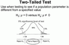
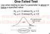
P Distributions: Confidence Interval: Normal Distribution (@)

A

(1) Confidence Interval: A range of values around an expected outcome. A random variable is expected to be within this range a certain percentage of the time.
(2) Example: the mean annual return (normally distributed) on a portfolio over many years is 11%, and the standard deviation of returns is 8%. Calculate a 95% confidence interval on next years return. —90% conf. int = Xbar+- 1.65s —95% conf. int = Xbar+- 1.96s —99% conf. int - Xbar +- 2.58s 11% +- (1.96((8%)=-4.7% to 26.7%

12
Q

P Distributions: Standard Normal Distribution

A

(1) A normal distribution that has been standardized has a mean of 0 and a standard deviation of 1. (2) To standardize a random variable, calculate the z-value. (3) Subtract the mean and divide by the standard deviation. z=X-mean/sd

13
Q

P Distributions: Calculating Probabilities Using the Standard Normal Distribution

A

Example: The EPS for a large group of firms are normally distributed an d have a u=$4.00 and a o=$1.50. Find the probability that a selected firm’s earnings are less than $3.70. z= 3.70-4.00/1.50-/20 3.60 is .2 sd below 4.00 mean. Check z table at .2 and .00. For negative z-table, calculate 10 - table value. There is a 42.07% probability that the EPS of a randomly selected form will be more than .20 sd below the mean Iess than $3.70.

14
Q

P Distributions: Shortfall risk and Roy’s Safety-First Ratio

A

(1) Shortfall risk: Probability that a portfolio return or value will be below a target return or value. (2) Rou’s Safety-First Ratio: Number of std. dev target is below expected expected return/value. (3) Example: Given the two portfolios, which has the lower probability of generating a return below 5%? —15-5)/12=/93 —18-4/25=.25

15
Q

P Distributions: Lognormal Distribution

A

(1) If x is normal, then e^x is lognormal. (2) Lognormal is always positive, used for modeling price relatives –> (1 +return= e^x

16
Q

P Distributions: Continuous Compounding

A

(1) Continuously compounding rate = ln(1 + HPR) (2) EAY with continuous compounding = e^i-1 (3) Example: 1-year holding period return = 8% —Continuous compounded rate of return = ln (1.08) = 7.7% —7.7% rate with continuous compounding, EAY = e^.077-1 = 8%

17
Q

P Distributions: Monte Carlo Simulation (5)

A

Simulation can be used to estimate a distribution of derivatives prices of NPVs (1) Specify distributions of random variables such as interest rates, underlying stock prices (2) Use computer random generation of variables (3) Value the derivative using those values (4) Repeat steps 2 and 3 1000s of times (5) Calculate mean/variance of all values.

18
Q

Sampling and Estimation: Sampling (4)

A

(1) To make inferences about parameters of a population we will use a sample (2) A simple random sample is one where every population member has an equal chance of being selected (3) A sampling distribution is the distribution of sample statistics for repeated sample size n. (4) Sampling error is the difference between a sample statistic and true population parameter.

19
Q

P Distributions: Historical Simulation (3)

A

(1) Similar to Monte Carlo simulation, but generates random variables from distributions of historical data. (2) Advantage: Don’t have to estimate distribution of risk factors (3) Disadvantage: Future outcomes for risk factors may be outside the historical range.

20
Q

Sampling and Estimation: Stratified Random Sampling (2)

A

(1) Create subgroups from population based on important characteristics (e.g. identify bonds according to callable, ratings, maturity, and coupon. (2) Selected samples from each subgroup in proportion to the size of the subgroup. —Used to construct bond portfolios to match a bond index or to construct a sample that has certain characteristics in common with the underlying population.

21
Q

Sampling and Estimation: Time-Series vs. Cross-Sectional Data (2)

A

(1) Time-series data: for example, monthly prices for IBM stocks for five years. (2)Cross-sectional data: for example, returns on all health care stocks last month

22
Q

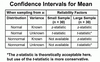
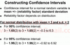
Sampling and Estimation: Central Limit Theorem (2)

A

(1) For any population with mean u and variance o^2, as the size of the random sample gets large, the distribution of sample means approaches normal distribution with a mean u and a varianve o2/n (2) Allows us to make inferences about and construct confidence intervals for population means based on sample means.

23
Q

Sampling and Estimation: Standard Error of the Sample Mean

A

(1) standard error of sample mean is the standard deviation of the distribution of sample means. (2) When population is known ox=o/sq.rt n When population is unknown sx =s/sq.rt n

24
Q

Sampling and Estimation: Standard Error of the Sample Mean-Example

A

(1) Example: The mean P/E for a sample of 41 firms is 19.0, and the standard deviation of the population is 6.6. What is the standard error of the sample mean? ox=o/sq.rt n = 6.6/sq.rt 41 = 1.03 (2) Interpretation: for sample size n=41, the distribution of the sample means would have a mean of 19.0 and a standard deviation of 1.03.

25
Q

Sampling and Estimation: Desirable Estimator Properties (3)

A

(1) Unbiased: expected value equal to parameter. (2) Efficient: sampling distribution has smallest variable of all unbiased estimators. (3) Consistent: larger sample –> better estimator, Standard error of estimate decrease with large sample size.

26
Q

Sampling and Estimation: Point Estimate and Confidence Interval

A

Example: The mean P/E point estimate for a sample of 41 firms is 19.0, and the standard error of the sample mean is 1.03, and the population is normal. —90% confidence interval is 19 +- 1.65(1.03) 17.3 < mean < 2.07 —95% confidence interval is 19 +- 1.96 (1.03 17.0 < mean < 21.0 —95 confidence interval for a randomly chosen firm (from population) is 19+- 1.96(6.6) or 6.06 < mean < 31.94

27
Q

Sampling and Estimation: Confidence Intervals for Mean

A

(1) When sampling from a normal distribution and known variance, always use z-statistic for reliability factors. (2) When sampling from a normal distribution and unknown variance, always use t-statistic for reliability factors.* (3) When sampling a nonnormal distribution and known variable, use z-statics for large samples (n>30). Reliability factors unknown for small samples. (4) When sampling a nonnormal distribution and unknown variance, use t-static for large sample. Reliability factors are unknown for small samples.* *z-statistics is theoretically acceptable, t is more conservative.

28
Q

Sampling and Estimation: Student’s t-distribution and degrees of freedom (4)

A

Properties of Student’s t-distribution (1) symmetrical (bell shaped) (2) Fatter tails than a normal distribution (3) Defined by a single parameter, degrees of freedom (df), where df=n-1 (4) As df increase, t-distribution approaches normal distribution (5) Lower degrees of freedom –> fatter tails

29
Q

Sampling and Estimation: T-Distributions

A
30
Q

Sampling and Estimation: Constructing Confidence Intervals

A
31
Q

Sampling and Estimation: Confidence Interval for Mean - Example

A

Example: Normal distribution, unknown variance: the sample mean is 19.0, the sample sd is 6.6, and n=41. establish a 90% confidence interval for the population mean. —t-table reliability factor is 1.684(df=40, a/2=.05) std. error of mean=s/sqrt of n= 6.6/sqrt 41= 1.03 19+-1.684(1.03=17.27 < mean < 20.73

32
Q

Sampling and Estimation: Sample Size Issues

A

We’ve seen that larger samples produce better estimates and small confidence intervals but: (1) Cost can be a factor- obtaining more data can increase costs, so there is a trade-off. (2) Including more data points from a population (time-period) with different parameters will not improve your estimate.

33
Q

Sampling and Estimation: Types of Bias (5)

A

(1) Data mining bias: from repeatedly doing tests on same data sample. (2) Sample selection bias: sample not really random. (3) Survivorship bias: sampling only surviving firms, mutual funds, hedge funds (4) Look-ahead bias: using information not available at the time to construct sample. (5) Time-period bias: relationship exists only during time period of sample data.

34
Q

Hypothesis Testing: Steps (7)

A

(1) State the hypothesis-relation to be tested (2) Select a test statistic (3) Specify the level of significance (4) State the decision rule for the hypothesis (5) Collect the sample and calculate statistics (6) Make a decision about the hypothesis (7) Make a decision based on test results.

35
Q

Hypothesis Testing: Null and Alternative Hypotheses (2)

A

(1) Null hypothesis H0 —The hypothesis to be tested —Researcher wants to reject it —Always includes the equal sign (2) Alternative hypothesis Ha —What the researcher would like to conclude —What is concluded if the researcher rejects the null hypothesis

36
Q

Hypothesis Testing: Test statistic and Critical Values (3)

A

(1) A test statistic is calculated from sample data, and compared to critical values to test H0 (2) If test statistics exceeds the critical value ( or is outside the range of critical values, the researcher rejects H0 (3) Critical values are like a confidence interval

37
Q

Hypothesis Testing: Two-tailed test

A

.

38
Q

Hypothesis Testing: One-tailed test

A

.

39
Q

Hypothesis Testing: Type I and Type II Errors

A

Type I Error:

  • Rejecting H0 when it is actually true
  • Significance level is Prob of type I Error

Type II Error:

  • Failing to reject H0 whenit is actually false
  • Power of test is 1- Prob of Type II Error
40
Q

Hypothesis Testing: Statistically vs. Economically Meaningful Result.

A

Statistical significance doe snot necessarily imply economic significance:

  • Tranactions costs
  • Taxes
  • Risk
41
Q

Hypothesis Testing: p-value Example

A

A p-value is the smallest level of significance at which the null can be rejected, the probability of getting the test statistic by chance if the null is true.

42
Q

Hypothesis Testing: Test Statistics: T-statistic

A

Test of mean of normal population when variance is unknown, use a t-statistic

43
Q

Hypothesis Testing: Test Statistics: Z-statistic

A

Test of mean of normal population when variance is known, use a z-statistic.

44
Q

Hypothesis Testing: Example

A

Test the hypothesis that fund’s mean return is equal to 1% per month at the 95% confidence (5% significance) level

Data provided:

  • Sample mean : 1.5%
  • Sample size: 45
  • Population standard deviation: 1.4%
  • Population distribution is non-normal
45
Q

Hypothesis Testing: Test Statistics: Difference in Means

A

Test of whether the means of two normal populations are equal- independent samples

46
Q

Hypothesis Testing: Paired Comparisons Test

A

Test of the difference between the means of two different populations- dependent samples

Paired Comparison Test

47
Q

Hypothesis Testing: Test Statistics

A

Note that the LOS only require you to:

Odentify the appropriate test statistic and interpret results for a hypothesis test concerning:

  1. The difference in means and the mean difference tests are t-tests, reject if t-stat is greater than critical value
  2. Use difference in means tests for samples from two independent normal populations
  3. Use mean differences test for two dependent, equal-size, samples from normal populations
48
Q

Hypothesis Testing: Test Statistics: Variance

A
49
Q

Hypothesis Testing: Test Statistics: F-Test

A

Test of whetehr the variances of two normal populations are equal is an F-test.

Putting the larger sample variance inthe numerator allows us to consider only upper critical value - although F-test is a two-tailed test.

50
Q

Hypothesis Testing: Parametric and Nonparametric Tests (2)

A
  • Parametric tests are based on assumptions about population distributions and popultion parameters (e.g. t-test, z-test, F-test)
  • Nonparametric tests make few if any assumptions about the popultaion distribution and test things other than parameter values (e.g., runs tests, rank correlation tests)
51
Q

Technical Analysis: Principles and Assumptions (3)

A
  • Stock values determined by supply and demand which are driven by both rational and irrational behavior
  • Technical analysts use price and trading volume to analyze changes in supply and demand
  • Security prices move in trends that persist for long periods and repeat themselves in predictable ways.
52
Q

Technical Analysis: Fundamental Analysis (2)

A
  • Fundamental analysts looks for changes in intrinsic values (what prices should be) based primarily on anticipated financial results and estimates of future cash flows
  • Technical analysts try to predict price change through analysis of past trades.
53
Q

Technical Analysis: Claimed Advantages (3)

A
  • It is based on actual trade data, whereas fundamental analysis is based on accounting numbers which can be estimates
  • Can be used for assets with no cash flows to be discounted for valuation (e.g. comodities)
  • Don’t have to learn accounting
54
Q

Technical Analysis: Disadvantages of Technical Analysis

A
  • May not work in illiquid markets
  • May not work in markets subject to manipulation (e.g. central bank currency intervention)
  • Bankrupt companies: Stock price →0, but short covering may create positive technical patterns
  • May not work at all if markets are weak-form efficient
55
Q

Technical Analysis: Line, Bar, and Volume Chart

A

.

56
Q

Technical Analysis: Point and Figure and Candlestick chart

A

.

57
Q

Technical Analysis: Trend Lines

A
  • Uptrend: Higher highs, higher lows
  • Downtrend: Lower highs, lower lows
58
Q

Technical Analysis: Support and Resistance

A
  • Support: Price when buying pressure limits a downtrend
  • Resistance: Price where selling pressure limits an uptrend

Examples of support and resistance:

  • Trendlines
  • Old highs, old lows
  • Round numbers, whole number prices
59
Q

Technical Analysis: Change in Polarity Principle (2)

A
  • Breached resistance levels become support
  • Breach support levels become resistance
60
Q

Technical Analysis: Reversal Patterns (4)

A

Reversal patterns: prior trend expected to reverse direction

  • Head and shoulders
  • Douple, triple top
  • Inverse head and shoulders
  • Double, triple bottom
61
Q

Technical Analysis: Continuation Patterns (4)

A

Continuation patterns: Prior trend expected to continue in same direction

62
Q

Technical Analysis: Price target

A

Price target for ensuing trend: Measure size of pattern, project from neckline

63
Q

Technical Analysis: Moving Averages

A
  • Moving average = Mean of last n prices
  • Larger n → Smoother moving average
64
Q

Technical Analysis: Bollinger Bands

A

Drawn above and below moving averages by # of std. dev., # of standard deviation determined by volatility

  • Short-term (contrarian)
    • Sell at top band - security overbought
    • Buy at bottom band - security oversold
  • Longer term
    • Buy on significant breakout above top band
    • Sell on significant breakout below lower band
65
Q

Technical Analysis: Bollinger Bands Price Chart

A
66
Q

Technical Analysis: Momentum Oscillators

A
  • Scaled price-based indicators
    • Oscillate around a value (e.g. 0 or 100)
    • Oscilalte between two values (e.g. 0 and 100)
  • Extreme values indicate overbough or oversold markets (contrarian trading signals.
  • Identify convergence or divergence of price movemet and oscillator movement
    • Convergence = continuation of trend
    • Divergence = early warning of change in trend
67
Q

Technical Analysis: Momentum Oscillators Price Chart

A
68
Q

Technical Analysis: Rate of Change (ROC) Oscillator

A

Also called a momentum oscillator

  • ROC = (Vt-Vt-n) x 100, oscillated around 0
  • ROC = Vt/Vt-n x 100, oscillates around 100

n is typically 10 days between prices

  • Buy signal: ROC crossed above 0 (100) during uptrend
  • Sell signal: ROC crosses below 0 (100) during dowwntrend
69
Q

Technical Analysis: Relative Strength Index (RSI)

A
70
Q

Technical Analysis: Stochastic Oscillator

A
71
Q

Technical Analysis: MACD

A
  • Two line: Moving Avg. Convergence/Divergence line and signal line
  • MACD = difference between two exponentially smoothed moving averages typically 12-day and 26-day
  • Signal line = Exponentially smoothed 9-day moving average of MACD
  • Oscillates around zero

MACD crosses above signal line= Buy

MACD crosses below signal line = Sell

72
Q

Technical Analysis: Sentiment Indicators (5)

A
  • Opinion polls
  • Put/call ratio
    • Put volume > call volume: Ratio > 1 →Negative sentiment
    • Call volume > put volume Ratio < 1 →Positive sentiment
    • Contrarian indicator
  • CBOE Volatility Index (VIX)
    • High when investors fear market decline
    • Contrarian indicator: investors bearish contrarians → bullish
  • Margin debt
  • Short interest ratio: # shares sold short/ total daily volume
73
Q

Technical Analysis: Flow of Funds Indicators

A
  • Short-term Trading Index (TRIN)

Activity in advancing stocks vs. activity in declining stocks

  • Margin debt
  • Mutual funds cash position:
    • Low in uptrends, high in downtrends
    • Fund cash is potential buying power → Contrarian indicator
  • New equity issuance, secondary offering
74
Q

Technical Analysis: Cycles

A
  • Kondratieff Wave: 54-year cycle
  • 18-year cycle
  • Decennial cycle: 10 years
  • Presidential cycle (U.S.): 4 years
    • 1st and 2nd year: worst performance
    • 3rd and 4th year: best performance
75
Q

Technical Analysis: Elliot Wave Theory

A
  • Market prices move in interconnected cycles that range from very short term to very long-term
  • Uptrends: 5 waves up, 3 waves down
  • Downtrends: 5 waves down, 3 waves up
  • Wave sizes conform to Fibonacci ratios
  • Fibonacci sequence: 0, 1, 1, 2, 3, 5, 8, 13, 21, 34, …
76
Q

Technical Analysis: Elliot Wave Theory Chart

A
77
Q

Technical Analysis: Intermarket Analysis

A

All markets are interrelated, influence each other

  • Equities, bonds, currencies, commodities
  • Industry groups: energy, utilities, consumar staples, healthcare, financial, info tech, materials, industrials, telecom, consumer discretionary
  • London, New York, Toyko, Hong Kong Germany

Relative strength charts show inflection points (e.g. equities/commodities, energy/S&P index, MSFT/info tech)