statistics notes 2020 march 30

Question 1

Data types

Answer 1

Categorical and numerical

Question 2

types of Categorical data

Answer 2

Nominal, Ordinal

Nominal:

Named data which can be separated into discrete categories which do not overlap.

Ordinal:

the variables have natural, ordered categories and the distances between the categories is not known.

Question 3

types of numerical data

Answer 3

Discrete, continuous

Question 4

Ordinal data

Answer 4

a categorical, statistical data type

the variables have natural, ordered categories and the distances between the categories is not known.

data which is placed into order or scale (no standardised value for the difference)

(easy to remember because ordinal sounds like order).

e.g.: rating happiness on a scale of 1-10. (no standardised value for the difference from one score to the next)

Question 5

Nominal Data mytutor.co.uk

Answer 5

Named data which can be

separated into discrete categories which do not overlap.

(e.g. gender; male and female) (eye colour and hair colour)

An easy way to remember this type of data is that nominal sounds like named,

nominal = named.

Question 6

Ordinal Data

mytutor.co.uk

Answer 6

Ordinal data:

placed into some kind of order or scale. (ordinal sounds like order).

e.g.:

rating happiness on a scale of 1-10. (In scale data there is no standardised value for the difference from one score to the next)

positions in a race (1st, 2nd, 3rd etc). (the runners are placed in order of who completed the race in the fastest time to the slowest time, but no standardised difference in time between the scores).

Intervaldata:

comes in the form of a numerical value where the differencebetween points is standardisedand meaningful.

Question 7

Interval Data

mytutor.co.uk

Answer 7

Interval data:

comes in the form of a numerical value where the difference between points is standardised and meaningful.

e.g.: temperature, the difference in temperature between 10-20 degrees is the same as the difference in temperature between 20-30 degrees.

can be negative

(ratio data can NOT)

Question 8

Ratio Data

mytutor.co.uk

Answer 8

Ratio data:

much like interval data – numerical values where the difference between points is standardised and meaningful.

it must have a true zero >> not possible to have negative values in ratio data.

e.g.: height be that centimetres, metres, inches or feet. It is not possible to have a negative height.

(comparing this to temperature (possible for the temperature to be -10 degrees, but nothing can be – 10 inches tall)

Question 9

inferential statistics

Answer 9

Population: an entire group of items, such as people, animals, transactions, or purchases >> Descriptive statistics applied if all values in the dataset are known.

>> not possible or feasible to analyse >>

Sample: a selected subset, called a sample, is extracted from the population.

The selection of the sample data from the population is random >> Inferential statistics applied >> develop models to extrapolate from the sample data to draw inferences about the entire population (while accounting for the influence of randomness)

Question 10

Quantitative analysis can be split into two major branches of statistics:

Answer 10

Descriptive statistics (if all values in the dataset are known)

Inferential statistics (extrapolates from the sample data to draw inferences about the entire population)

Question 11

inferential

Answer 11

következtetési, deductive

Question 12

Descriptive statistical analysis

Answer 12

As a critical distinction from inferential statistics, descriptive statistical analysis applies to scenarios where all values in the dataset are known.

Question 13

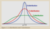
Confidence, confidence level

Answer 13

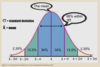
Confidence is a measure to express how closely the sample results match the true value of the population.

Confidence level: 0% - 100%

95%: if we repeat the experiment numerous times (under the same conditions), the results will match that of the full population in 95% of all possible cases.

Question 14

Hypothesis Testing

Answer 14

Hypothesis test:

evaluate two mutually exclusive statements to determine which statement is correct given the data presented.

incomplete dataset >> hypothesis testing is applied in inferential statistics to determine if there’s reasonable evidence from the sample data to infer that a particular condition holds true of the population.

Question 15

null hypothesis

Answer 15

A hypothesis that the researcher attempts or wishes to “nullify.”

most of the world believed swans were white, and black swans didn’t exist inside the confines of mother nature. The null hypothesis that swans are white

The term “null” does not mean “invalid” or associated with the value zero.

Question 16

In hypothesis testing, the null hypothesis (H0)

Answer 16

In hypothesis testing, the null hypothesis (H0) is assumed to be the commonly accepted fact but that is simultaneously open to contrary arguments.

If substantial evidence to the contrary >> the null hypothesis is disproved or rejected >> the alternative hypothesis is accepted to explain a given phenomenon.

Question 17

The alternative hypothesis

Answer 17

The alternative hypothesis is expressed as Ha or H1.

Covers all possible outcomes excluding the null hypothesis.

Question 18

What is the relationship between the null hypothesis and alternative hypothesis?

Answer 18

null hypothesis and alternative hypothesis are mutually exclusive,

which means no result should satisfy both hypotheses.

Question 19

a hypothesis statement must be

Answer 19

a hypothesis statement must be clear and simple. Hypotheses are also most effective when based on existing knowledge, intuition, or prior research.

Hypothesis statements are seldom chosen at random. a good hypothesis statement should be testable through an experiment, controlled test or observation.

(Designing an effective hypothesis test that reliably assesses your assumptions is complicated and even when implemented correctly can lead to unintended consequences.)

Question 20

A clear hypothesis

Answer 20

A clear hypothesis tests only one relationship and avoids conjunctions such as “and,” “nor” and “or.”

A good hypothesis should include an “if” and “then” statement

(such as: If [I study statistics] then [my employment opportunities increase])

Question 21

The good hypothesis sentence structure

Answer 21

The first half of this sentence structure generally contains an independent variable (this is the hypothesys) (i.e., if study statistics) in the

second half: a dependent variable (whatyou’re attempting to predict) (i.e., employment opportunities).

Question 22

A dependent variable represents

Answer 22

A dependent variable represents what you’re attempting to predict,

2nd half of the hypothesys sentence

Question 23

The independent variable is

Answer 23

The independent variable (in the first half of the sentence) is the variable, that supposedly impacts the outcome of the dependent variable (which is the 2nd half of the hypothesys senetence)

Question 24

double-blind

Answer 24

where both the participants and the experimental team aren’t aware of who is allocated to the experimental group and the control group respectively.

Question 25

probability

Answer 25

probability expresses the likelihood of something happening expressed in percentage or decimal form; typically expressed as a number with a decimal value called a floating-point number.

Question 26

odds

Answer 26

odds define the likelihood of an event occurring with respect to the number of occasions it does not occur.

For instance, the odds of selecting an ace of spades from a standard deck of 52 cards is 1 against 51. On 51 occasions a card other than the ace of spades will be selected from the deck.

Question 27

correlation

Answer 27

Correlation is often computed during the exploratory stage of analysis to understand general relationships between variables.

Correlation describes the tendency of change in one variable to reflect a change in another variable.

Question 28

confounding variable

Answer 28

the observed correlation could be caused by a third and previously unconsidered variable,

aka lurking variable or confounding variable.

It’s important to consider variables that fall outside your hypothesis test as you prepare your research and before publishing your results.

Question 29

zavarba hoz

Answer 29

confound

Question 30

the curse of dimensionality

Answer 30

confusing correlation and causation arises when you analyze too many variables while looking for a match.

(In statistics, dimensions can also be referred to as variables).

If we are analyzing three variables, the results fall into a three-dimensional space.)

You can find instances of the “curse” or phenomenon using Google Correlate (www.google.com/trends/correlate)

the curse of dimensionality tends to affect machine learning and data mining analysis more than traditional hypothesis testing due to the high number of variables under consideration. e.g:

…It turns out that the bang energy drink, for example, came onto the market at a similar time as Alibaba Cloud’s international product offering and then grew at a similar pace in terms of Google search volume..

átok

Question 31

Data

Answer 31

A term for any value that describes the characteristics and attributes of an item that can be moved, processed, and analyzed.

The item could be a transaction, a person, an event, a result, a change in the weather, and infinite other possibilities.

Data can contain various sorts of information, and through statistical analysis, these recorded values can be better understood and used to support or debunk a research hypothesis.

Question 32

 Population

Answer 32

The parent group from which the experiment’s data is collected,

e.g., all registered users of an online shopping platform or all investors of cryptocurrency.

Question 33

Sample

Answer 33

A subset of a population collected for the purpose of an experiment,

e.g., 10% of all registered users of an online shopping platform or 5% of all investors of cryptocurrency. 

A sample is often used in statistical experiments for practical reasons, as it might be impossible or prohibitively expensive to directly analyze the full population.

Question 34

Variable

Answer 34

A characteristic of an item from the population that varies in quantity or quality from another item,

e.g., the Category of a product sold on Amazon.

A variable that varies in regards to quantity and takes on numeric values is known as a quantitative variable,

e.g., the Price of a product.

A variable that varies in quality/class is called a qualitative variable,

e.g., the Product Name of an item sold on Amazon.

This process is often referred to as classification, as it involves assigning a class to a variable.

Question 35

Variable types (what is the term for the process to establish types?)

Answer 35

quantitative variable (varies in regards to quantity and takes on numeric values),

qualitative variable (varies in quality/class),

classification

Question 36

Discrete Variable

Answer 36

A variable that can only accept a finite number of values,

e.g., customers purchasing a product on Amazon.com can rate the product as 1, 2, 3, 4, or 5 stars. In other words, the product has five distinct rating possibilities, and the reviewer cannot submit their own rating value of 2.5 or 0.0009.

Helpful tip: qualitative variables are discrete,

e.g. name or category of a product.

Question 37

Continuous Variable

Answer 37

A variable that can assume an infinite number of values,

e.g., depending on supply and demand, gold can be converted into unlimited possible values expressed in U.S. dollars.

A continuous variable can also assume values arbitrarily close together.

e.g.: price and reviews (number of reviews on a product) are continuous variables

Question 38

Categorical Variables

Answer 38

A variable whose possible values consist of a discrete set of categories,

rather than numbers quantifying values on a continuous scale)

(such as gender or political allegiance,

Question 39

Ordinal Variables

Answer 39

(a subcategory of categorical variables),

ordinal variables categorize values in a logical and meaningful sequence.

ordinal variables contain an intrinsic ordering or sequence such as {small; medium; large} or {dissatisfied; neutral; satisfied; very satisfied}.

The distance of separation between ordinal variables does not need to be consistent or quantified. (For example, the measurable gap in performance between a gold and silver medalist in athletics need not mirror the difference in performance between a silver and bronze medalist.)

standard categorical variables, i.e. gender or film genre,

Question 40

Independent and Dependent Variables

Answer 40

An independent variable (expressed as X) is the variable that supposedly impacts the dependent variable (expressed as y).

For example, the supply of oil (independent variable) impacts the cost of fuel (dependent variable).

As the dependent variable is “dependent” on the independent variable, it is generally the independent variable that is tested in experiments. As the value of the independent variable changes, the effect on the dependent variable is observed and recorded. 

In analyzing Amazon products, we could examine Category, Reviews and 2-Day Delivery as the independent variables and observe how changes in those variables affect the dependent variable of Price. Equally, we could select the Reviews variable as the dependent variable and examine Price, 2-Day Delivery and Category as the independent variables and observe how these variables influence the number of customer reviews.

Question 41

What determines wether a variable is “independent” or “dependent” ?

Answer 41

The labels of “independent” and “dependent” are hence determined by experiment design rather than inherent composition

(one variable could be a dependent variable in one study and an independent variable in another)

Question 42

two events are considered independent if …

Answer 42

In probability,

two events are considered independent if the occurrence of one event does not influence the outcome of another event

(the outcome of one event, such as flipping a coin, doesn’t predict the outcome of another. If you flip a coin twice, the outcome of the first flip has no bearing on the outcome of the second flip)

Question 43

P(E|F)

Answer 43

the probability of E given F

The probability of one event (E) given the occurrence of another conditional event (F) is expressed as P(E|F),

Question 44

two events are said to be independent if ..

Answer 44

Conversely, two events are said to be independent if

P(E|F) = P(E).

This equation holds that the probability of E is the same irrespective of F being present.

This expression can also be tweaked to compare two sets of results where the conditional event (F) is absent from the second trial.

Question 45

Bayes’ theorem in nutshell

Answer 45

The premise of this theory is to find the probability of an event, based on prior knowledge of conditions potentially related to the event.

Bayes’ theorem “is to the theory of probability what the Pythagorean theorem is to geometry.” 

For instance, if reading books is related to a person’s income level, then, using Bayes’ theory, we can assess the probability that a person enjoys reading books based on prior knowledge of their income level.

In the case of the 2012 U.S. election, Nate Silver drew from voter polls as prior knowledge to refine his predictions of which candidate would win in each state. Using this method, he was able to successfully predict the outcome of the presidential election vote in all 50 states.

Question 46

Triboluminescence

Answer 46

Triboluminescence is the light emitted when crystals are crushed…”

‘When you take a lump of sugar and crush it with a pair of pliers in the dark, you can see a bluish flash. Some other crystals do that too.

lump - csomó

pliers - fogó

Question 47

Bayes’ theorem formula

Answer 47

P(A/B)= P(A) * P(B/A) / P(B) 

P(A|B) is the probability of A given that B happens (conditional probability)

P(A) is the probability of A (without any regard to whether event B has occurred (marginal probability)

P(B|A) is the probability of B given that A happens (conditional probability)

P(B) is the probability of B without any regard to whether event A has occurred (marginal probability) 

Bayes’ theorem can be written in multiple formats including the use of ∩ (intersection) instead of P(B/A).

https://www.dropbox.com/s/p8io6kx4d4d0vne/Bayes%20theorem%20formula.png?dl=0

Question 48

conditional probability (and what is opposite?)

Answer 48

Both P(A|B) and P(B|A)

are the conditional probability of observing one event given the occurrence of the other.

Both P(A) and P(B)

are marginal probabilities, which is the probability of a variable without reference to the values of other variables.

Question 49

Let’s imagine a particular drug test is 99% accurate at detecting a subject as a drug user.

Suppose now that 5% of the population has consumed a banned drug.

How can Bayes’ theorem be applied to determine the probability that an individual, who has been selected at random from the population is a drug user if they test positive?

Answer 49

we need to designate A and B events:

P(A): real drug user probability and

P(B): probability of identifying someone as positive (even if in reality is not >> all real positives from users and the false positives from non-users)

P(A/B): this is the question; probability of a realdruguseridentified positivelyinthetest

(different from 0.99 because there is a probability, that the test shows false positive result from non-users

(the test does not catch all positives either, but not important now)

P(A): probability of a real“drug user” >> 0.05 (implies probability of non-user: 1-0.05 = 0.95)

P(B/A): probability of a positivetest>> 0.99 (result given that the individual is a drug user)

P(B): the probability of a positivetestresult(two elements: actually identified real users + false positively identified non-users): 0.059

1. actually identified real users: 0.05 * 0.99 = 0.0495
2. false positively identified non users; (1-0.05) * 0.01 = 0.95 * 0.01= 0.9505 * 0.01=0.0095

0.059= 0.0495 + 0.0095 (from 1. + 2.)

P(A/B) = P(A) * P(B/A) / P(B) >> 0.05 * 0.99 / 0.059 = 0.8389

P(user|positive test) = P(user) * P(positive test|user)/P(positive test)

Bayes theorem example 1

Question 50

What is the implication of the false positive test results? How to deal with it?

Answer 50

Using Bayes’ theorem, we’re able to determine that (in the current example) there’s an 83.9% probability that an individual with a positive test result is an actual drug user.

The reason this prediction is lower for the general population than the successful detection rate of actual drug users or P (positive test | user), which was 99%,

is due to the occurrence of false-positive results.

Question 51

Bayes’ theorem weakness

Answer 51

important to acknowledge that Bayes’ theorem can be a weak predictor in the case of poor data regarding prior knowledge and this should be taken into consideration.

Question 52

Binomial Probability

Answer 52

used for interpreting scenarios with two possible outcomes.

(Pregnancy and drug tests both produce binomial outcomes in the form of negative and positive results, and so too flipping a two-sided coin.)

The probability of success in a binomial experiment is expressed as p, and the number of trials is referred to as n.

Question 53

drawing aggregated conclusions from multiple binomial experiments such as flipping consecutive heads using a fair coin?

Answer 53

you would need to calculate the likelihood of multiple independent events happening,

which is the product (multiplication) of their individual probabilities

Question 54

Permutations

Answer 54

tool to assess the likelihood of an outcome.

not a direct metric of probability,

permutations can be calculated to understand the total number of possible outcomes, which can be used for defining odds.

calculate the full number of permutations, which refers to the maximum number of possible outcomes from arranging multiple items

Question 55

find the full number of seating combinations for a table of three

Answer 55

we can apply the function three-factorial,

which entails multiplying the total number of items by each discrete value below that number,

i.e., 3 x 2 x 1 = 6.

Question 56

Four-factorial is

Answer 56

Four-factorial is

4 x 3 x 2 x 1 = 24

Question 57

you want to know the full number of combinations for randomly picking a box trifecta,

which is a scenario where you select three horses to fill the first three finishers in any order.

Answer 57

using permutations is for horse betting;

we’re calculating the total number of permutations

and also a

subset of desired possibilities (recording a 1st place, recording a 2nd place, and recording a 3rd place finish).

The total number of combinations on where each horse can finish is calculated as Twenty-factorial

We next need to divide twenty-factorial by

seventeen-factorial to ascertain all possible combinations of a top three placing.

Twenty-factorial / Seventeen-factorial = 6,840

Thus, there are 6,840 possible combinations among a 20-horse field that will offer you a box trifecta.

Question 58

CENTRAL TENDENCY

Answer 58

the central point of a given dataset,

aka central tendency measures.

the three primary measures of central tendency are the mean, mode, and median.

Question 59

The Mean

Answer 59

Arithmetic mean (sum divided by the sample number)

the midpoint of a dataset, is

the average of a set of values and the easiest central tendency measure to understand.

sum of all numeric values / by the number of observations

Question 60

trimmed mean

Answer 60

the mean can be highly sensitive to outliers.

(statisticians sometimes use the trimmed mean, which is the mean obtained after removing extreme values at both the high and low band of the dataset,

such as removing the bottom and top 2% of salary earners in a national income survey).

Question 61

The Median

Answer 61

the median pinpoints the data point(s) located in the middle of the dataset to suggest a viable midpoint.

The median, therefore, occurs at the position in which exactly half of the data values are above and half are below when arranged in ascending or descending order.

The solution for an even number of data points is to calculate the average of the two middle points

Question 62

The Median or mean is better?

Answer 62

The mean and median sometimes produce similar results, but, in general,

the median is a better measure of central tendency than the mean for data that is asymmetrical as it is less susceptible to outliers and anomalies.

The median is a more reliable metric for skewed (asymmetric) data

Question 63

The Mode

Answer 63

statistical technique to measure central tendency

The mode is the data point in the dataset that occurs most frequently.

Question 64

discrete categorical values

Answer 64

a variable that can only accept a finite number of values

Question 65

ordinal values

Answer 65

the categorization of values in a clear sequence

(such as a 1 to 5-star rating system on Amazon)

Question 66

Why The Mode is advantageous?

Answer 66

easy to locate in datasets with a low number of discrete

categorical values (a variable that can only accept a finite number of values) or

ordinal values (the categorization of values in a clear sequence)

Question 67

Why can be The Mode is disadvantageous?

Answer 67

The effectiveness of the mode can be arbitrary and depends heavily on the composition of the data.

The mode, for instance, can be a poor predictor for datasets that do not have a single high number of common discrete outcomes (all star values have about the same %)

Question 68

Weighted Mean

Answer 68

statistical measure of central tendency factors the

weight of each data point to analyze the mean.

used when you want to emphasize a particular segment of data without disregarding the rest of the dataset.

e.g.: students’ grades, the final exam accounting for 70% of the total grade.

Question 69

What is the a suitable measure of central tendency?

Answer 69

depends on the composition of the data.

The mode: easy to locate in datasets with a low number of discrete values or ordinal values,

The mean and median: suitable for datasets that contain continuous variables.

The weighted mean: used when you want to emphasize a particular segment of data without disregarding the rest of the dataset.

Question 70

MEASURES OF SPREAD

Answer 70

describes how data varies

The composition of two datasets can be very different despite the fact they each dataset has the same mean.

The critical point of difference is the range of the datasets, which is a simple measurement of data variance.

Question 71

range of the datasets

Answer 71

As the difference between the highest value (maximum) and the lowest value (minimum),

the range is calculated by subtracting the minimum from the maximum.

knowing the range for the dataset can be useful for data screening and identifying errors.

An extreme minimum or maximum value, for example, might indicate a data entry error, such as the inclusion of a measurement in meters in the same column as other measurements expressed in kilometers.

Question 72

Standard Deviation

Answer 72

describes the extent to which individual observations differ from the mean.

the standard deviation is a measure of the spread or dispersion among data points just as important as central tendency measures for understanding the underlying shape of the data.

Question 73

How Standard deviation measures variability ?

Answer 73

Standard deviation measures variability

by calculating the average squared distance of all data observations from the mean of the dataset.

Question 74

Standard Deviation what low/high SD values mean?

Answer 74

the lower the standard deviation, the less variation in the data

When SD is a lower number (relative to the mean of the dataset) >> it indicates that most of the data values are clustered closely together,

whereas a higher value indicates a higher level of variation and spread.

a low or high standard deviation value depends on the dataset (depends on the mean, on the range and even on the variability of the values in the dataset )

SD -1.png

Question 75

How to Calculate Standard Deviation ?

Answer 75

SD-2

Question 76

histogram

Answer 76

visual technique for interpreting data variance is to plot the dataset’s distribution values

Question 77

what is standard normal distribution?

Answer 77

A normal distribution with a

mean of 0 and a

standard deviation of 1

Question 78

What histogram shape a normal distribution produces?

Answer 78

data is distributed evenly >> a bell curve

A symmetrical bell curve of a standard normal model

bell curve -1.png

Question 79

Normal distribution can be transformed to a standard normal distribution by ..

Answer 79

converting the original values to standardized scores

Question 80

normal distribution features:

Answer 80

• the highest point of the dataset occurs at the mean (x̄).
• the curve is symmetrical around an imaginary line that lies at the mean.
• at its outermost ends, the curves approach but never quite touch or cross the horizontal axis.
• the location at which the curves transition from upward to downward cupping (known as inflection points) occur one standard deviation above and below the mean.

bell curve -1.png

Question 81

how variables diverge in the real world?

Answer 81

The symmetrical shape of normal distribution is a often reasonable description.

(body height, IQ tests, variable values generally gravitate towards a symmetrical shape around the mean as more cases are added)

Question 82

Empirical Rule

Answer 82

variables often diverge in the real world like a

The symmetrical shape of normal distribution

Question 83

How the Empirical Rule describes normal distribution ?

Answer 83

Approximately 68% of values fall within one standard deviation of the mean.

Approximately 95% of values fall within two standard deviations of the mean.

Approximately 99.7% of values fall within three standard deviations of the mean.

Aka the 68 95 99.7 Rule or the Three Sigma Rule

Question 84

What the French mathematician Abraham de Moivre discovered?

Answer 84

Following an empirical experiment flipping a two-sided coin, de Moivre discovered that

an increase in events (coin flips) gradually leads to a symmetrical curve of binomial distribution.

Question 85

What is Binomial distribution?

Answer 85

It describes a statistical scenario when only one of two mutually exclusive outcomes of a trial is possible,

i.e., a head or a tail, true or false.)

Question 86

Total possible outcomes of flipping a head with four standard coins

Flipping exp. with 4 coins..

Answer 86

the histogram has five possible outcomes

the probability of most outcomes is now lower.

the more data >> the histogram contorts into a symmetrical bell-shape.

As more data is collected >> more observations settle in the middle of the bell curve, a smaller proportion of observations land on the left and right tails of the curve.

The histogram eventually produces approximately 68% of values within one standard deviation of the mean.

Using the histogram, we can pinpoint the probability of a given outcome such as two heads (37.5%) and whether that outcome is common or uncommon compared to other results—a potentially useful piece of information for gamblers and other prediction scenarios.

It’s also interesting to note that the mean, median, and mode all occur at the same point on the curve as this location is both the symmetrical center and the most common point. However, not all frequency curves produce a normal distribution.

symm bell shape in binom distrib.png

Question 87

MEASURES OF POSITION

Answer 87

on a normal curve there’s a decreasing likelihood of replicating a result the further that observed data point is from the mean.

We can also assess whether that data point is approximately

one (68%), two (95%) or three standard deviations (99.7%) from the mean.

This, however, doesn’t tell us the probability of replicating the result.

we want to identify the probability of replicating a result.

Question 88

How to identify the probability of replicating a result?

Answer 88

Depending on the size of the dataset: Z-Score

Question 89

Z-Score

Answer 89

finds the distance from the sample’s mean to an individual data point expressed in units of standard deviation.

z-score.png

Question 90

Z-Score is 2.96, means ..

Answer 90

the data point is located 2.96 standard deviations from the mean in the positive direction.

This data point could also be considered an anomaly as it is close to three deviations from the mean and different from other data points.

Question 91

Z-Score is -0.42, means ..

Answer 91

the data point is positioned 0.42 standard deviations from the mean in the negative direction,

(this data point is lower than the mean)

Question 92

anomaly

Answer 92

if the Z-Score falls three positive or negative deviations from the mean (in case of normal distribution) >> anomaly

>> data points that lie an abnormal distance from other data points. >> a rare event that is abnormal and perhaps should not have occurred.

in the case of a normal distribution if the Z-Score falls three positive or negative deviations from the mean of the dataset, it falls beyond 99.7% of the other data points on a normal distribution curve.

sometimes viewed as a negative exception, such as fraudulent behavior or an environmental crisis.

help to identify data entry errors and are commonly used in fraud detection to identify illegal activities.

Question 93

Outliers

no unified agreement on how to define outliers, but:

Answer 93

data points that diverge from primary data patterns as outliers because they record unusual scores on at least one variable and are more plentiful than anomalies.

Question 94

Z-Score applies to..

Answer 94

to a normally distributed sample

with a known standard deviation of the population.

Question 95

When to use T-Score?

Answer 95

sometimes the mean isn’t normally distributed or the

standard deviation of the population is unknown or not reliable,

<< which could be due to insufficient sampling (small sample size)

Question 96

What is the problem with small datasets?

Answer 96

The standard deviation of small datasets is susceptible to change as more observations are included

Question 97

T-Score who, when discovered, how else called?

Answer 97

Irish statistician W. S. Gosset. early 20th Century published under the pen name“Student” >>

sometimes called “Student’s T-distribution.”

Question 98

What Z-Score/ T-Score using?

Answer 98

Z-distribution / T-distribution (Student’s T-distribution)

Question 99

What is Z-Score and T-Score primary function?

Answer 99

same primary function (measure distribution) they’re used with different sizes of sample data.

Question 100

What is Z-distribution?

Answer 100

standard normal distribution

Question 101

What Z-Score measures?

Answer 101

the deviation of an individual data point from the mean for datasets with 30 or more observations

based on Z-distribution (standard normal distribution).

Z and T distribution graph.png

Question 102

T-distribution features

Answer 102

the T-distribution is not one fixed bell curve rather its distribution curve changes (multiple shapes) in accordance with the size of the sample.

• if the sample size is small, (e.g. 10): >> the curve is relatively flat with a high proportion of data points in the curve’s tails.
• as the sample size increases >> the distribution curve approaches the standard normal curve (Z-distribution) with more data points closer to the mean at the center of the curve.

Z and T distribution graph.png

Question 103

A standard normal curve is defined by…

Answer 103

by the 68 95 99.7 rule,

which sets approximate confidence levels for one, two, and three standard deviations from a mean of 0.

Based on this rule, 95% of data points will fall 1.96 standard deviations from the mean

Question 104

if the sample’s mean = 100 and we randomly select an observation from the sample (in case of standard normal curve)..

Answer 104

the probability of that data point falling within 1.96 standard deviations of 100 is 0.95 or 95%.

To find the exact variation of that data point from the mean we can use the Z-Score

Question 105

In the case of smaller datasets we need to..

what is the problem?

Answer 105

they don’t follow a normal curve—we instead need to use the T-Score.

Question 106

T-Score

Answer 106

The formula is similar to that of the Z-Score,

except the standard deviation is divided by the sample size.

Also, the standard deviation is that of the sample in question, which may or may not reflect that of the population (when more observations are added to the dataset).

T-score.png

Question 107

You’ll want to use the t score formula when ..

Answer 107

when you don’t know the population standard deviation and you have a small sample (under 30).

Question 108

T-score formula

Answer 108

T-score formula.png

Question 109

When to use T-score formula ?

Answer 109

You’ll want to use the t score formula when you don’t know the population standard deviation and you have a small sample (under 30).

Question 110

What is the T Score in essence?

Answer 110

A t score is one form of a standardized test statistic

(the other you’ll come across in elementary statistics is the z-score).

The t score formula enables you to take an individual score and transform it into a standardized form > one which helps you to compare scores.

Question 111

Z-score tells you:

Answer 111

z score tells you how many standard deviations from the mean your score is

Question 112

very good website >> work out here

Answer 112

https://www.statisticshowto.datasciencecentral.com/probability-and-statistics/z-score/

Question 113

Z score = 0: what is the meaning?

Answer 113

Your observation is right in the middle of the distribution (in the mean)

Question 114

Z score = 1: what is the meaning?

Answer 114

Your observation is 1 SD away from the mean (above if +1, bellow if -1)

Question 115

Z-score summary

Answer 115

Z-score summary.png

Question 116

The Law of Large Numbers

Answer 116

if we take a sample (n) observations of our random variable & avg the observation (mean)–

it will approach the expected value E(x) of the random variable.

Question 117

What is a typical sample size that would allow for usage of the central limit theorem?

Answer 117

In practice, “n = 30” is usually what distinguishes a “large” sample from a “small” one.

In other words, if your sample has a size of at least 30 you can say it is approximately Normal (and, hence, use the Normal distribution).

If, on the other hand, your sample has a size less than 30, it’s best to use the t-distribution instead.

Question 118

Do we average large number of samples when applying Central limit theorem?

Answer 118

We are not averaging a large number of samples, rather, we are obtaining the averages from many repeated samples.

The distribution of the sample averages is the Normal distribution we obtained.

It does not represent the original distribution well. But it’s not supposed to do so!

This Normal distribution is the distribution of the sample mean. Its use it to let us talk about the probability of the sample mean being in a given interval, better understanding the population mean,

and so forth.

Question 119

How can we use the Central Limit Theorem?

Answer 119

We can get info about a population

not taking large number of samples, but

getting the averages from many repeated smaller samples

>> their distribution will be normal (around the mean)

>> this normal distribution is the distribution of the sample mean.

>> population mean can be determined

>> can determine the probability of the sample mean being in a given interval

(and maybe more what I still dont get)

Question 120

Central Limit Theorem

Answer 120

if we take the mean of the samples (n) and plot the frequencies of their mean,

>> we get a normal distribution! as the sample size (n) increases –> approaches infinity –> we find a normal distribution

(calculate the mean of a few random samples (e.g: n=4) from the whole population > gives a value (sample mean) > repeat several times with the same sample size (4-4-4 samples) > plot their means on a frequency distribution > if you do it many times > the distribution of the sample means will follow normal distribution

if the sample size is low (e g.: n=4) >> the curve will be wide and flat

as sample size increases (e g.: n >>> 4) > the curve will be higher and tighter around the mean

Central Limit Theorem .png

Question 121

what’s the difference between an average and mean?

Answer 121

The word ‘average’ is a bit more ambiguous.

Average can legitimately mean almost any measure of central tendency: mean, median, mode, typical value, etc.

However, even “mean” admits some ambiguity, as there are different types of means.

The one you are probably most familiar with it the arithmetic mean, although there is

also a geometric mean and a harmonic mean.

Question 122

Skew and Kurtosis of the Normal Distribution

Answer 122

Skew and Kurtosis of the Normal Distribution .png

Question 123

opposite of fraction number

Answer 123

integer

Question 124

The Standard Error of the Mean

Answer 124

the Standard Error of the Mean

the Stand Dev of the Mean

the ‘stand deviation’ of the ‘sample distribution’ of the ‘sample mean’

–> all the same

the Standard Error of the Mean.png

Question 125

what is ‘mu’ and ‘X upper lined’

Answer 125

the whole population can be characterized by a mean μ (mu),

but it is impossible to measure (everybody) so we take

several samples from the whole population and calculate the sample means x̄ (x upper lined)

according to the Central Limit Theorem the means of the taken samples will follow Normal distribution

even if the distribution is not normal in the population

Question 126

what is sigma squared?

Answer 126

population variance

Question 127

what is sigma ?

Answer 127

population SD

Question 128

what is ‘s’ squared?

Answer 128

sample variance

Question 129

what is ‘s’ ?

Answer 129

sample SD (square rooted sample variance)

but square rooting is non -linear >> square rooting (n-1) >> introduces slight errors, still the best we have

sample standard deviation.png

Question 130

sample standard deviation

Answer 130

sample SD (square rooted sample variance)

but square rooting is non -linear >> square rooting (n-1) >> introduces slight errors, still the best we have sample

standard deviation.png

Question 131

Variance

Answer 131

squared standard deviation

square root of variance gives –> standard deviation

population variance / population variance:

the differences of sample values and means squared –>

summed up –> divided by sample number (n; in case of population variance) or (n-1; sample variance)

population variance: sigma

sample variance: ‘s’

Variance.png

Question 132

difference between one-tailed test and 2 tailed test

Answer 132

one-tailed test considers one direction of results (left or right) from the null hypothesis,

whereas a two-tailed test considers both directions (left and right).

the objective of the hypothesis test is not to challenge the null hypothesis in one particular direction but to consider both directions as evidence of an alternative hypothesis.

there are two rejection zones, known as the critical areas.

Results that fall within either of the two critical areas trigger rejection of the null hypothesis and thereby validate the alternative hypothesis.

1 tailed test-1.png

2 tailed test-1.png

Question 133

Type I Error in hypothesis testing

Answer 133

the rejection of a null hypothesis (H0) that was true and should not have been rejected.

This means that although the data appears to support that a relationship is responsible,

the covariance of the variables is occurring entirely by chance. (this does not prove that a relationship doesn’t exist, merely that it’s not the most likely cause)

covariance: a measurement of how related the variance is between two variables

This is commonly referred to as a false-positive.

Question 134

Type II Error in hypothesis testing

Answer 134

accepting a null hypothesis (H0) that should’ve been rejected because

the covariance of variables was probably not due to chance.

This is also known as a false-negative.

covariance: a measurement of how related the variance is between two variables

Question 135

pregnancy test example for

type I

type II errors

Answer 135

we need to establish a H0 what can be challenged experimentally

we can do test for pregnancy -> if the test shows pregnancy -> we can reject H0 stating that the woman is not pregnant –>>

the null hypothesis (H0): the woman is not pregnant.

H0 rejected if the woman is pregnant –> H0 is false and

H0 accepted if the woman is not pregnant (H0 is true).

the test may not be 100% accurate >> mistakes may occur.

If H0 rejected (false + test) and the woman is not actually pregnant (H0 is true), this leads to a Type I Error.

If H0 is accepted (the test fails to show pregnancy, false negative) and the woman is pregnant (H0 is false) –> this leads to a Type II Error

(we do not reject H0 > accept H1)

Question 136

example for hypothesis testing my take (not sure)

Answer 136

we change sg –> causing effect or not? let’s detect events to see

H0: no affect

H1: does have affect

–> if we can detect events, wich would be highly unlikely by chance (e.g. three SD away from the random distribution mean)

ez az otletem, de majmeglattyuk

Question 137

What is Covariance?

Answer 137

a measure of the variance between two variables.

covariance is a measure of the relationship between two random variables.

a measurement of how related the variance is between two variables

The metric evaluates how much – to what extent – the variables change together.

However, the metric does not assess the dependency between variables.

Covariance summed

Question 138

covariance is measured..

Answer 138

covariance is measured in units.

The units are computed by multiplying the units of the two variables. The variance can take any positive or negative values.

The values are interpreted as follows:

Positive covariance: Indicates that two variables tend to move in the same direction.

Negative covariance: Reveals that two variables tend to move in inverse directions.

Covariance summed

Question 139

covariance concept is used..

Answer 139

In finance, the concept is primarily used in portfolio theory.

One of its most common applications in portfolio theory is the diversification method,

using the covariance between assets in a portfolio.

By choosing assets that do not exhibit a high positive covariance with each other,

the unsystematic risk can be partially eliminated

Covariance summed

Question 140

the covariance between two random variables X and Y can be calculated using the following formula (for population):

Answer 140

Covariance summed

Question 141

Covariance measures what?

what are the limitations of covariance?

Answer 141

Covariance measures the total variation of two random variables

from their expected values.

Using covariance, we can only gauge the direction of the relationship (whether the variables tend to move in tandem or show an inverse relationship)

it does not indicate the strength of the relationship,

nor the dependency between the variables.

Covariance summed

Question 142

Correlation measures

Answer 142

Correlation measures the strength of the relationship between variables.

Correlation is the scaled measure of covariance.

It is dimensionless.

In other words, the correlation coefficient is always a pure value and not measured in any units.

correlation:

covariance divided by standard deviation of both X and Y variables

Covariance summed

Question 143

investing Example of Covariance

Answer 143

John is an investor. His portfolio primarily tracks the performance of the S&P 500 and John wants to add the stock of ABC Corp. Before adding the stock to his portfolio, he wants to assess the directional relationship between the stock and the S&P 500.

John does not want to increase the unsystematic risk of his portfolio.

Thus, he is not interested in owning securities in the portfolio that tend to move in the same direction.

John can calculate the covariance between the stock of ABC Corp. and S&P 500 by following the steps below:

https://corporatefinanceinstitute.com/resources/knowledge/finance/covariance/

Question 144

Why Statistical Significance important?

Answer 144

Given that the sample data cannot be truly reliable and representative of the full population, there is the possibility of a sampling error or random chance affecting the experiment’s results.

not all samples randomly extracted from the population are preordained to reproduce the same result. It’s natural for some samples to contain a higher number of outliers and anomalies than other samples, and naturally, results can vary.

If we continued to extract random samples, we would likely see a range of results and the mean of each random sample is unlikely to be equal to the true mean of the full population.

Question 145

statistical significance : what is the role?

Answer 145

outlines a threshold for rejecting the null hypothesis.

Statistical significance is often referred to as the p-value (probability value) and is expressed between 0 and 1.

Question 146

what is the meaning of p-value of 0.05?

Answer 146

A p-value of 0.05, expresses a 5% possibility of replicating a result if we take another sample.

Question 147

how we use the p-value in hypothesis testing?

Answer 147

the p-value is compared to a pre-fixed value (the alpha).

If the p-value returns as

equal or less than alpha, then the result is statistically significant and we can reject the null hypothesis.

If the p-value is greater than alpha, the result is not statistically significant and we cannot reject the null hypothesis.

Alpha sets a fixed threshold for how extreme the results must be before rejecting the null hypothesis.

(alpha should be defined before the experiment and not after the results have been obtained)

Question 148

How is alpha for two-tailed tests?

Answer 148

For two-tailed tests, the alpha is divided by two.

Thus, if the alpha is 0.05 (5%), then the critical areas of the curve each represent 0.025 (2.5%).

Hypothesis tests usually adopt an alpha of between 0.01 (1%) and 0.1 (10%), there is no predefined or optimal alpha for all hypothesis tests.

Question 149

Why is there a tendency to set alpha to a low value such as 0.01?

Answer 149

alpha is equal to the probability of a Type I Error (incorrect rejection of the H0 due to false positive)

(when the result falls into the alpha% critical (rejection) zone(s)..

when the result is in the critical zone (defined by alpha) -> the H0 rejected –> tendency to minimalize the critical zone by decreasing it’s size choosing smaller alpha

(incorrect rejection of the null hypothesis) the critical area is smaller >> less chance of incorrectly rejecting H0

but!

increases the risk of a Type II Error (incorrectly accepting the null hypothesis) because

the critical zone will be so tiny, that no value can fall into it anymore –> can not reject the HO –> incorrect acceptance of H0

>> inherent trade-off in hypothesis testing >> most industries have found that 0.05 (5%) is the ideal alpha for hypothesis testing

Question 150

What is alpha equal to?

Answer 150

alpha is equal to the probability of a Type I Error

(incorrect rejection of the null hypothesis) (false positive result)

Question 151

Confidence in essence

Answer 151

Confidence is

a statistical measure of prediction confidence regarding whether

the sample result of the experiment is true of the full population

Question 152

Confidence is calculated as

Answer 152

Confidence is calculated as (1 – α).

if the alpha is 0.05 >> confidence level of the experiment is 0.95 (95%).

1.0 – α = confidence level 1.0 – 0.05 = 0.95

Question 153

Confidence relation to alpha

Answer 153

Confidenceis calculated as (1 – α).

if the alphais 0.05>> confidencelevel of the experiment is 0.95 (95%).

1.0 – α = confidence level 1.0 – 0.05 = 0.95

Question 154

What alpha of 0.05 tells and

what not?

Answer 154

alpha = 0.05

–> reject the null hypothesis when the results are in a 5% zone, but

this doesn’t tell us where to plant the null hypothesis rejection zone(s). >> we need to define the critical areas set by alpha.

two-tail test with two confidence intervals and two critical areas .png

Question 155

For what wee need to define the critical areas set by alpha?

Answer 155

for the null hypothesis rejection zone(s)

Question 156

How to define the critical areas set by alpha?

Answer 156

Confidence intervals define the confidence bounds of the curve

Two-tailed test:

two confidence intervals define two critical areas outside the upper and lower confidence limits;

One-tailed test:

a single confidence interval defines the left/right-hand side critical area.

two-tail test with two confidence intervals and two critical areas .png

Question 157

Confidence intervals define..

Answer 157

Confidence intervals define the confidence bounds of the curve

Question 158

types of hypothesis test

Answer 158

left one-tailed, right one-tailed, two-tailed

Question 159

Normal distribution sufficient sample data (n>30) what formula for a two-tailed test ?

Answer 159

Z: Z-distribution critical value (found using a Z-distribution table)

formula for a two-tailed test.png

Question 160

Z-Statistic is used to find..

Answer 160

The Z-Statistic is used

to find the distance between the null hypothesis and the sample mean.

Question 161

How do you utilize Z-Statistic in hypothesis testing?

Answer 161

In hypothesis testing, the experiment’s Z-Statistic is compared with the expected statistic (critical value) for a given confidence level.

Z-Statistic is used to find the distance between the null hypothesis and the sample mean.

Question 162

Example teenage gaming habits in Europe; data given: n=100 (100 teens) mean (of gaming time): 22 hrs

Stand. Dev.= 5.7 (calculated) alpha of 0.05

how to find the confidence intervals for 95%?

Using a two-tailed test what can you find out?

Answer 162

95% certain that our sample data will fall somewhere between 20.8828 and 23.1172 hours.

Example teenage gaming habits in Europe

Question 163

Example teenage gaming habits in Europe;

data given: now low sample size (10) n=10 (10 teens)

mean (of gaming time): 22 hrs Stand. Dev.= 5 (calculated) alpha of 0.05

How to find the confidence intervals for 95%?

Using a two-tailed test what can you find out?

Answer 163

T-distribution Confidence Intervals can be found

T-distribution Confidence Intervals Xsample.png

Question 164

the overall objective of hypothesis testing is

Answer 164

to prove that the outcome of the sample data is representative of the full population and not occurring by chance caused by randomness in the sample data.

Question 165

Hypothesis testing four steps:

Answer 165

1: Identify the null hypothesis

(what you believe to be the status quo and wish to nullify)

and the type of test (i.e. one-tailed or two-tailed).

2: State your experiment’s alpha

(statistical significance and the probability of a Type I Error) and set the confidence interval(s).

3: Collect sample data and conduct a hypothesis test.
4: Compare the test result to the critical value

(expected result) and decide if you should support or reject the null hypothesis.

Question 166

What Z-Score measures?

Answer 166

the distance between a data point and the sample’s mean

Question 167

What Z-Score measures in hypothesis testing?

Answer 167

in hypothesis testing,

we use the Z-Statistic to find the distance between a sample mean and the null hypothesis.

Question 168

How Z-Statistic is expressed?

what is the meaning?

Answer 168

numerically

the higher the statistic, the higher the discrepancy between the sample data and the null hypothesis.

Z-Statistic of close to 0 means the sample mean matches the null hypothesis—confirming the null hypothesis pegged to a p-value, which is the probability of that result occurring by chance.

hypothesis testing

Question 169

Z-Statistic of close to 0 means

Answer 169

Z-Statistic of close to 0 means the sample mean matches the null hypothesis—confirming the null hypothesis

Question 170

rögzítve van

Answer 170

pegged to

Question 171

What p<0.05 indicates?

Answer 171

A low p-value, such as 0.05, indicates that the sample mean is unlikely to have occurred by chance.

a p-value of 0.05 is sufficient to reject the null hypothesis

Question 172

How to find the p-value for a Z-statistic?

Answer 172

To find the p-value for a Z-statistic,

we need to refer to a Z-distribution table

Z-distribution table .png

z Critical Value.png

Question 173

What a two-Sample Z-Test compares?

Answer 173

A two-sample Z-Test compares the difference between the means of two independent samples with a known standard deviation.

(we assume: the data is normally distributed and a minimum of 30 observations)

Question 174

what is high enough Z value

(Z-Statistic value)?

Answer 174

what is high enough Z value (Z-Statistic value)? >>

depends on the level of confidence (determined by alpha)

and the type of the test (one tailed or two tailed) >>

can be found in tables finding the critical Z-value >>

shows in the table the level of confidence

e.g. in a Two-Sample Z-Test

Question 175

What do you calculate with a Two-Sample Z-Test?

Answer 175

a Z value (Z-Statistic value)

it helps to evaluate the null hypothesis (e.g.: a difference between two sets of values (two samples), we need to calculated the SD of the two samples > it shows what extent they very > it helps to see if the difference between the two groups is due to variation or real)

if Z is close to O >> the sample mean matches the null hypothesis >> confirms the null hypothesis (so the two samples are equal, the difference found between their means is due to chance (coming from variation)

if Z is high enough >> reject H0 so reject that µ1 = µ2 (mu1 = mu2) >> accept H1 (the means of samples are indeed different)

what is high enough Z value (Z-Statistic value)? >> depends on the level of confidence (alpha) and the type of the test (one tailed or two tailed) >> can be found in tables finding the critical Z-value >> shows in the table the level of confidence in tables the critical Z-value can be found: these Z values should be used in confidence interval calculations when a confidence level is determined -by alpha- we need to see the corresponding critical Z-value (find in tables) >> this sets the limit where the H0 can be rejected

Two-Sample Z-Test formula.png

z Critical Value.png

Question 176

z Critical Value

Answer 176

z Critical Value.png

Question 177

One-Sample Z-Test example:

Company A claims their new phone battery outperforms

former 20 hrs time.

30 users

mean battery life (sample of 30 users) >> 21 hours,

SD= 3

is 21 > 20 if the SD=3 and n=30’ ?

Answer 177

One-Sample Z-Test

Question 178

Two-Sample Z-Test practical:

Company A claims their phone battery outperforms Company B. 60 users mean battery life (Company A) (sample of 30 users) >> 21 hours, SD= 3

mean battery life (Company A) (sample of 30 users) >> 19 hours, SD= 2

is that claim right?

Answer 178

Two-Sample Z-Test.png

Question 179

One-Sample Z-Test in essence

Answer 179

one-sample only (sample size: 30) (I guess it is the min) calculate SD

assume norm. distribution

calculate mean >> is it different from a value?

not comparing two samples, only one sample’s mean compared to a value

Question 180

One-Sample Z-Test

Answer 180

one-sample only (sample size: 30) (I guess it is the min) calculate SD assume norm. distribution calculate mean >> is it different from a value? (not comparing two samples, only one sample’s mean compared to a value

One-Sample Z-Test formula

Question 181

One-Sample Z-Test formula

Answer 181

One-Sample Z-Test formula.png

Question 182

What do you do if you need to compare two mean values coming from two different samples?

(n=30 min and normal distribut with calculated SD)

Answer 182

Two-Sample Z-Test.png

Question 183

T-Test in essence

Answer 183

Similar to the Z-Test,

a T-Test analyzes the distance between a sample mean and the null hypothesis but is based on T-distribution (using a smaller sample size) and

uses the standard deviation of the sample rather than of the population.

Question 184

The main categories of T-Tests:

Answer 184

• An independent samples T-Test (two-sample T-Test) for comparing means from two different groups,

such as two different companies or two different athletes.

This is the most commonly used type of T-Test.

• A dependent sample T-Test (paired T-test) for comparing means from the same group at two different intervals,
  i. e. measuring a company’s performance in 2017 against 2018.
• A one-sample T-Test for testing the sample mean of a single group against a known or hypothesized mean.

Question 185

What is T-Statistic?

Answer 185

The output of a T-Test called the T-Statistic

quantifies the difference between the sample mean and the null hypothesis.

As the T-Statistic increases in the +/- direction, the gap between the sample data and null hypothesis expands.

we refer to a T-distribution table

Question 186

If we have a one-tailed test with an alpha of 0.05 and sample size of 10 (df 9), what can we expect?

Answer 186

we can expect 95% of samples to fall within 1.83 standard deviations of the null hypothesis.

T-distribution table.png

Question 187

Sample (n=10) >> Mean, SD calculated >> we carry out T-Test:

If our sample mean returns a T-Statistic greater than the critical score of 1.83, what can we conclude?

Answer 187

we can conclude the results of the sample are statistically significant and unlikely to have occurred by chance—allowing us to reject the null hypothesis.

H0: mu= (a certain) value (so the mean is different from that value, the difference we found is not due to a chance, but genuine

T-distribution table.png

Question 188

What is the T-Statistic critical score (for 95% confidence)?

Answer 188

for a one-tail test: T-Statistic must be greater than the critical score of 1.83 for 95% confidence (alpha=0.05)

for a two-tail test: T-Statistic critical score: 2.26 for 95% confidence (alpha=0.05/2 = 0.025) two critical areas would each account for 2.5% of the distribution based on 95% confidence with confidence intervals of -2.262 and +2.262 from the null hypothesis.

T Table

Question 189

Independent Samples T-Test in essence

Answer 189

An independent samples T-Test compares means from two different groups.

Independent Samples T-Test formula.png

Question 190

What is Pooled standard deviation used for?

Answer 190

part of a greater calculation for Independent Samples T-Test calculation

https://www.dropbox.com/s/48mecjisbglgbbn/Independent%20Samples%20T-Test%20formula.png?dl=0

Question 191

Independent Samples T-Test Xmpl

comparecustomer spending between the

desktopversion of their website andthe mobilesite.

25desktop customers spent an average of $70with a SD of $15.

mobileusers, 20customers spent $74on average with a SD of $25.

We test the difference of the sample mean and the known mean using a two-tail test with an alpha of 0.05 (95% confidence).

Answer 191

Independent Samples T-Test.png

Question 192

What to do if we want to: compare customer spending between the desktop version of their website and the mobile site. 25 desktop customers spent an average of $70 with a SD of $15. mobile users, 20 customers spent $74 on average with a SD of $25.

Answer 192

Independent Samples T-Test

Independent Samples T-Test.png

Question 193

Dependent Sample T-Test in essence

Answer 193

A dependent sample T-Test is used for comparing means from the same group at two different intervals.

Dependent Samples T-Test formula.png

Question 194

What to use if we want to compare means from the same group at two different intervals (at two different timepoints, but same players)

Answer 194

Dependent Samples T-Test

Dependent Samples T-Test.png

Question 195

Dependent Sample T-Test what for?

Answer 195

if we want to compare means from the same group at two different intervals (at two different timepoints, but same players)

Dependent Samples T-Test.png

Question 196

One-Sample T-Test in essence

Answer 196

A one-sample T-Test is used for testing the sample mean of a single group against a known or hypothesized mean.

One-Sample T-Test formula.png

Question 197

When Z-Test is used for hypothesis testing?

what is it based on?

Answer 197

A Z-Test, is

used for datasets with 30 or more observations (normal distribution) with a known standard deviation of the population and is calculated based on Z-distribution.

Question 198

When T-Test is used for hypothesis testing?

Answer 198

A T-Test is used in scenarios when you have a small sample size or you don’t know the standard deviation of the population

and you instead use the standard deviation of the sample and T-distribution.

Question 199

What to do, if you want to compare small sample sized sample (group) and you do not know the SD of the whole population (only of your small sized sample’s)?

Answer 199

T-Test is used in scenarios when you have a small sample size or you don’t know the standard deviation of the population and you instead use the standard deviation of the sample and T-distribution.

You can test if the sample mean is the same with sg. (it will be a hypothesis)

(H null: they are the same, H1: they are different)

you can test H0 with T-test >> you get T-Statistics value >> lookup the critical value in the T-distribution table >> compare them >> accept/reject the null hypothesis

Question 200

What T-Test is used for ?

Answer 200

small sample size or you don’t know the standard deviation of the population instead use the standard deviation of the sample and T-distribution

You can test if the sample mean is the same with sg. (it will be a hypothesis) (H null: they are the same, H1: they are different) you can test H0 with T-test >> you get T-Statistics value >> lookup the critical value in the T-distribution table >> compare them >> accept/reject the null hypothesis

Question 201

What technique is used to compare experimental group and a control group (placebo)?

Answer 201

hypothesis testing for comparing two proportions from the same population population expressed in percentage form,

i.e. 40% of males vs 60% of females.

we need to conduct a ‘two-proportion Z-Test’

https://www.dropbox.com/s/3ml84x5fhon19gj/Two-proportion%20Z-Test.png?dl=0

Question 202

two-proportion Z-Test’

Answer 202

hypothesis testing for comparing two proportions from the same population population expressed in percentage form,

i.e. 40% of males vs 60% of females.

we need to conduct a ‘two-proportion Z-Test’ to compare experimental group and a control group (placebo)

https://www.dropbox.com/s/3ml84x5fhon19gj/Two-proportion%20Z-Test.png?dl=0

Question 203

Two-proportion Z-Test practical

Answer 203

Two-proportion Z-Test practical

Two-proportion Z-Test practical.png

We consider a new energy drink formula proposes to improve students’ test scores.

max test score: 1600 (the average score is 1050 - 1060). Evaluation: whether the students’ results exceed 1060 points.

sample of 2,000 students split evenly into an exp. group (energy drink) and a ctrl group (placebo). Results:

Ctrl Group = 500 exceeded /1000

Exp Group = 620 exceeded /1000; looks more than 500 > real difference?

Question 204

in Two-proportion Z-Test we get Z-Statistic value: how do we evaluate it?

Answer 204

Critical areas of 2.5% on each side of the two-tailed (normal distribution) curve from a distance of 1.96 standard deviations.

If the Z-Statistic falls within 1.96 standard deviations of the mean (within the 95% area) >>

we can conclude that the proportions of the ‘experimental test’ and ‘control test’ results were equal (the exp. group and the ctrl group are not different)

If the Z-Statistic falls out of the 95% area >> reject null hypothesis (the proportions are not the same) >> so they are different (H1 is true)

Normal distribution curve with marked critical areas.png

Question 205

We consider a new energy drink formula proposes to improve students’ test scores. max test score: 1600 (the average score is 1050 - 1060). Evaluation: whether the students’ results exceed 1,060 points. sample of 2,000 students split evenly into an exp. group (energy drink) and a ctrl group (placebo). Results: Ctrl Group = 500 surpassed /1000 Exp Group = 620 surpassed/1000; looks more than 500 > real difference? How to evaluate the difference?

Answer 205

Two-proportion Z-Test

Two-proportion Z-Test practical.png

Question 206

What is the null hypothesis when comparing exp. group with a ctrl group?

Answer 206

two-proportion Z-Test based on the following hypotheses:

H0: p1 = p2 (The proportions are the same with the difference equal to 0)

H1: p1 ≠ p2 (The two proportions are not the same)

we detect a difference between the two groups >> is it a real difference (or just due to chance)?

we want to find out >> H0: we state, that they are the same (this hypothesis we want to nullify,reject >> we can reject, if the Z-test value will fall into an area of the distribution, where there is less than 5% chance that would fall by chance considering the variation in that sample group

we anchor the null hypothesis with the statement that we wish to nullify:

(the two proportions of results are identical and it just so happened that the results of the experimental group different that of the control group due to a random sampling error) <– if reject, H1 is true: they are not equal

in general:

H0: the known, the status quo, what we want to chalenge

H0: (equal, not equal, less, more)

H1: the opposite, engulfing eveything else

Two-proportion Z-Test practical.png

Question 207

What is the meaning if we define confidence level = 95% ?

H0: p1 = p2 (The proportions are the same with the difference equal to 0)

H1: p1 ≠ p2 (The two proportions are not the same)

Answer 207

H0: p1 = p2 (The proportions are the same with the difference equal to 0)

H1: p1 ≠ p2 we test it; (The two proportions are not the same) << if it occurs less than 5% by chance (the probability that it happens is more than 95% that not by chance) ->we reject H0, because 95% probility holds that not equal

putting other way: actually the formula examines the difference between the two sample proportions

H0: p1-p2=0

Ha: p1-p2≠0 we test it; (The two proportions are not the same -> the difference of the proportions is not zero; if the probality that it is zero by chance is less than 5% -> 95% -or more- probability that not by chance -> so it is genuinely true) << if it occurs less than 5% by chance (the probability that it happens is more than 95%)

we’ll reject the null hypothesis if there’s a less than 5% chance of the alternative hypothesis occurring by chance.

we anchor the null hypothesis with the statement that we wish to nullify:

(e.g.: exp group-placebo group test: the two proportions of results are identical and it just so happened that the results of the experimental group different that of the control group due to a random sampling error)

Normal distribution curve with marked critical areas.png

Question 208

regression analysis essence

Answer 208

technique in inferential statistics it is used to test how well a variable predicts another variable.

the term “regression” is derived from Latin, meaning “going back”

Question 209

What is the the objective of regression analysis ?

Answer 209

The objective of regression analysis is to find a line that best fits the data points on the scatterplot to make predictions.

Linear regression, the line is straight and cannot curve or pivot.

Nonlinear regression, meanwhile, grants the line to curve and bend to fit the data.

Question 210

trendline

Answer 210

trendline

A straight line cannot possibly intercept all data points on the scatterplot > linear regression can be thought of as a trendline visualizing the underlying trend of the dataset.

hyperplane:

a perpendicular line from the regression line to each data point on the scatterplot >> the aggregate distance of each point would equate to the smallest possible distance to the hyperplane.

Question 211

hyperplane

Answer 211

a perpendicular line from the regression line to each data point on the scatterplot

>> the aggregate distance of each point would equate to the smallest possible distance to the hyperplane.

Question 212

coefficient

Answer 212

slope aka. coefficient in statistics.

the term “coefficient” is generally used over “slope” in cases where there are multiple variables in the equation (multiple linear regression) and the line’s slope is not explained by any single variable.

Question 213

slope

Answer 213

The slope of a regression line (b) represents the rate of change in y as x changes.

Because y is dependent on x > the slope describes the predicted values of y given x.

The slope of a regression line is used with a t-statistic to test the significance of a linear relationship between x and y.

The slope can be found by referencing the hyperplane;

(scatterplots in statistics) as one variable increases, the other variable increases by the average value denoted by the hyperplane.

The slope is useful in forming predictions.

Question 214

How do you calculate slope?

(I did not get this)

Answer 214

With ordinary least squares method

(one of the most common linear regressions) slope, is found by calculating

b as the covariance of x and y,

divided by the variance (sum of squares) of x,

The slope must be calculated before the y-intercept when using a linear regression, as

the intercept is calculated using the slope.

slope calculation formula.png

Question 215

How is the slope useful? example..

Answer 215

We can use the slope, in forming predictions.

to predict a child’s height based on his parents’ midheight

(the intercept between parents’ midheight (X) of 72 inches and a son’s expected height (y)

>> the y value is approximately 71 inches.

Predicted height of a child whose parents’ midheight.png

Question 216

Regression analysis is useful for..

Answer 216

Regression analysis

(aka regression towards the mean) is a useful method for estimating relationships among variables testing if they’re somehow related.

Linear regression is not a fail-proof method of making predictions,

the trendline does offer a primary reference point to make estimates about the future.

Question 217

linear regression summary bbas

Answer 217

The regression model (and a scatter chart)

excellent tool to depict the relationship between two variables. Provides a visual representation and a mathematical model that relates the two variables.

describes the relation between x;y in a scatter plot

y = mx + b

(m: slope; b: intercept)

calculates m and b in such a way, that minimizes the distance (error) of the points from the regression line on the plot

(more accurately: reduce the sum of the errors squared >> “least squares regression” name)

linear regression summary bbas.png

Question 218

Linear regression Xmple

Answer 218

Linear regression Xmple.png

Question 219

What is R-squared for?

Answer 219

If we apply Linear regression analysis to large datasets with a higher degree of scattering or three-dimensional and four-dimensional data, hard to validate the trendline only by looking at it > A mathematical solution to this problem is to apply R-squared (the coefficient of determination)

Question 220

R-squared

Answer 220

(the coefficient of determination)

R-squared is a test to see what level of impact the independent variable has on data variance.

R-squared (a number between 0-1 (produces a percentage value)

0% : the linear regression model accounts for none of the data variability in relation to the mean (of the dataset) >> the regression line is a poor fit (for the given dataset)

100% : the linear regression model expresses all the data variability in relation to the mean (of the dataset) >> the regression line is a perfect fit mathematical solution to validate the (calculated) relationship in the regression model

defines the percentage of variance in the linear model in relation to the independent variable.

Question 221

How R-squared is calculated?

Answer 221

R² is a ratio ->

-> division needed to be calculated: SSR/SST

R-squared is calculated as

the sum of square regression (SSR) divided by

the sum of squares total (SST) -> SSR/SST

SSR: calculated from the regression analysis given theoretical values for the dependent variable (y’); y’ based on the y’=mx+b formula

it is the total sum of

[the individual values calculated for each datapoint from the theoretical (y’) and the actual/measured y̅ mean values at each point] -> squared -> sum up

SSR= (y’ - y̅)²

(y’ - y̅)² calculated for each datapoint and summed up and squared to get SSR

SST: calculated from the actual measured values of y and the mean of actual y values

it is the total sum of

[the individual values calculated for each datapoint from the actual y values (y) and the actual y̅ mean values at each point] -> squared -> sum up

SSR= (y - y̅)²

(y - y̅)² calculated for each datapoint and summed up and squared to get SSR

R-squared calculation.png

Question 222

Pearson Correlation in essence

Answer 222

A common measure of association between two variables.

Describes the strength or absence of a relationship between two variables.

Slightly different from linear regression analysis, which expresses the average mathematical relationship between two or more variables with the intention of visually plotting the relationship on a scatterplot.

Pearson correlation is a statistical measure of the co-relationship between two variables without any designation to independent and dependent qualities.

Question 223

Interpretations of Pearson correlation coefficients

Answer 223

Pearson correlation (r) is expressed as a number (coefficient) between -1 and 1.

-1 denotes the existence of a strong negative correlation

0 equates to no correlation, and

+1 for a strong positive correlation.

a correlation coefficient of -1 means that for every positive increase in one variable, there is a negative decrease of a fixed proportion in the variable

(airplane fuel which decreases in line with distance flown)

a correlation coefficient of 1 signifies an equivalent positive increase in one variable based on a positive increase in another variable

(food calories of a particular food that goes up with its serving size)

a correlation coefficient of zero notes that for every increase in one variable, there is neither a positive or negative change (the two variables aren’t related)

Interpretations of Pearson correlation coefficients.png

Question 224

Pearson correlation coefficients xmpl

Answer 224

Describes the strength or absence of a relationship between two variables

Pearson correlation coefficients xmpl.png

Question 225

Clustering analysis in essence

Answer 225

clustering analysis aims

to group similar objects (data points) into clusters based on the chosen variables.

This method partitions data into assigned segments or subsets (where objects in one cluster resemble one another and are dissimilar to objects contained in the other cluster(s).

Objects can be interval, ordinal, continuous or categorical variables.

(a mixture of different variable types can lead to complications with the analysis because the measures of distance between objects can vary depending on the variable types contained in the data)

Question 226

Regression and clustering

Answer 226

Regression and clustering shown on a scatterplot.png

Question 227

clustering analysis is used in

Answer 227

developed originally from anthropology,

psychology (later) 1930-s

personality psychology (1943)

today: in data mining, information retrieval, machine learning, text mining, web analysis, marketing, medical diagnosis, and many more

Specific use cases include analyzing symptoms, identifying clusters of similar genes, segmenting communities in ecology, and identifying objects in images.

not one fixed technique rather a family of methods, (includes hierarchical clustering analysis and non-hierarchical clustering)

Question 228

Hierarchical Clustering Analysis

Answer 228

(HCA) is a technique

to build a hierarchy of clusters.

An example: divisive hierarchical clustering, which is a top-down method where all objects start as a single cluster and are split into pairs of clusters until each object represents an individual cluster.

Hierarchical Clustering Analysis.png

Question 229

Agglomerative hierarchical clustering

Answer 229

a bottom-up method of classification (more popular approach)

Carried out in reverse each object starts as a standalone cluster a hierarchy is created by merging pairs of clusters to form progressively larger clusters.

three steps:

1. Objects start as their own separate cluster, which results in a maximum number of clusters.
2. The number of clusters is reduced by combining the two nearest (most similar) clusters. (differentiate by the interpretation of the “shortest distance” )
3. This process is repeated until all objects are grouped inside one single cluster.

>> hierarchical clusters resemble a series of nested clusters organized within a hierarchical tree.

Question 230

What is the difference between “agglomerate clustering” and “ divisive clustering”?

Answer 230

The agglomerate cluster starts with a broad base and a maximum number of clusters.

The number of clusters falls at subsequent rounds until there’s one single cluster at the top of the tree.

In the case of divisive clustering, the tree is upside down. At the bottom of the tree is one single cluster that contains multiple loosely related clusters. These clusters are sequentially split into smaller clusters until the maximum number of clusters is reached. Hierarchical clustering >> dendrogram chart to visualize the arrangement of clusters. (they demonstrate taxonomic relationships and are commonly used in biology to map clusters of genes or other samples)

(Greek dendron - “tree.”)

Nearest neighbor and a hierarchical dendrogram.png

Question 231

Agglomerative Clustering Techniques

Answer 231

Various methods

(differ in both the technique -to find the “shortest distance” between clusters- and in the shape of the clusters they produce)

Nearest Neighbor

The furthest neighbor

Average aka UPGMA (Unweighted Pair Group Method with Arithmetic Mean)

Centroid Method

Ward’s Method

Question 232

Nearest neighbor

Answer 232

creates clusters based on the distance between the two closest neighbors.

you find the shortest distance between two objects

>> combine them into one cluster >> repeated

>> the next shortest distance between two objects is found

(either expands the size of the first cluster or forms a new cluster between two objects)

Question 233

Furthest Neighbor Method

Answer 233

Produces clusters by measuring the distance between the most distant pair of objects. The distance between each possible object pair is computed

>> the object pairs located furthest apart are unable to be linked.

At each stage of hierarchical clustering, the two closest objects are merged into a single cluster.

Sensitive to outliers.

Question 234

Average aka UPGMA

Answer 234

(Unweighted Pair Group Method with Arithmetic Mean)

Merges objects by calculating the distance between two clusters and measuring the average distance between all objects in each cluster and joining the closest cluster pair.

Initially, no different to nearest neighbors because the first cluster to be linked contains only one object. Once a cluster includes two or more objects > the average distance between objects within the cluster can be measured which has an impact on classification.

Question 235

Centroid Method

Answer 235

Utilizes the object in the center of each cluster (centroid) to determine the distance between two clusters.

At each step, the two clusters whose centroids are measured to be closest together are merged.

Question 236

Ward’s Method

Answer 236

Draws on the sum of squares error (SSE) between two clusters over all variables to determine the distance between clusters.

All possible cluster pairs are combined >> the sum of the squared distance across all clusters is calculated. At each round attempts to merge two separate clusters by combining the two clusters that best minimize SSE >> The pair of clusters that return the highest sum of squares is selected and conjoined.

Produces clusters relatively equal in size (may not always be effective).

Can be sensitive to outliers.

One of the most popular agglomerative clustering methods in use today.

Question 237

Measures of Distance why important?

Answer 237

Measurement method >>

different method >>

different distance >>

lead to different classification results >>

impact on cluster composition

Measures of Distance.png

Question 238

Distance measurement methods

Answer 238

Euclidean distance

(standard across most industries, including machine learning and psychology)

Squared Euclidean distance

Manhattan distance (reduces the influence of outliers and resembles walking a city block)

Maximum distance, and

Mahalanobis (internal cluster distances tend to be emphasized (distances between clusters are less significant).

Manhattan distance versus Euclidean distance.png

Question 239

Euclidean distance formula

Answer 239

Euclidean distance formula.png

Question 240

Nearest Neighbor Exercise

Answer 240

Nearest Neighbor Exercise.png

Question 241

Non-Hierarchical Clustering methods

Answer 241

(Partitional clustering) different from hierarchical clustering and is commonly used in business analytics.

Divide n number of objects into m number of clusters (rather than nesting clusters inside large clusters).

Each object can only be assigned to one cluster and each cluster is discrete (unlike hierarchical clustering) >> no overlap between clusters and

no case of nesting a cluster inside another. >>

usually faster and require less storage space than hierarchical methods >>

(typically used in business scenarios)

Helps to select the optimal number of clusters to perform classification (rather than mapping the hierarchy of relationships within a dataset using a dendrogram chart)

Non-Hierarchical Clustering methods.png

Question 242

Example of k-means clustering

Answer 242

Example of k-means clustering.png

Question 243

k-means clustering in a nutshell and downsides

Answer 243

attempts to split data into k number of clusters

not always able to reliably identify a final combination of clusters

(need to switch tactics and utilize another algorithm to formulate your classification model)

measuring multiple distances between data points in a three or four-dimensional space (with more than two variables) is much more complicated and time-consuming to compute its

success depends largely on the quality of data and

there’s no mechanism to differentiate between relevant and irrelevant variables;

the variables you selected are relevant and especially if chosen from a large pool of variables

Question 244

What are Measures of Spread?

Answer 244

(measures of dispersion)

how wide the set of data is

The most common basic measures are:

The range

(including the interquartile range and the interdecile range)

(how much is in between the lowest value (start) and highest value (end)

(interquartile range, which tells you the range in the middle fifty percent of a set of data)

The standard deviation

square root of variance

a measure of how spread out data is around center of the distribution (the mean).

gives you an idea of where, percentage wise, a certain value falls.

e.g. you score one SD above the mean on a test (normally distributed -bell shaped). >> your score puts you in the top 84% of test takers)

The variance

a very simple statistic, gives an extremely rough idea of how spread out a data set is. As a measure of spread, it’s actually pretty weak. A large variance, doesn’t tell you much about the spread of data — other than it’s big!

The most important reason the variance exists >> to find the SD

SD squared >> variance

Quartiles

divide your data set into quarters according to where those numbers falls on the number line.

not very useful on its own >> used to find more useful values like the interquartile range

Question 245

how to insert unicode character symbols?

Answer 245

x with overline [x̅]:

Type the x then go to Insert >

Symbol

In the Character Viewer select Unicode from the left list

[You may have to click the ✲ to Customize the List]

Select Combining Diacritical Marks in the top middle pane

Locate & double-click the Overline [U-0305] in the lower middle pane

how to insert unicode character symbols.png

Question 246

Variance summary

Answer 246

Variance summary.png

Question 247

population mean character

Answer 247

mu

Question 248

sample mean character

Answer 248

x bar (x overline)

Question 249

population variance character

Answer 249

sigma squared

Question 250

sample variance character

Answer 250

s squared

Question 251

frequency distribution

Answer 251

a table dividing the data intro groups (classes) shows how many data values occur in each group

Question 252

Summary of clustering types

Answer 252

Summary of clustering types.png

Question 253

Not everyone has cancer, who has the symptoms (only 1 out of 10.000) >>

1/10.000 healthy individuals have the same symptoms worldwide but they do not have cancer

What is the probability that a patient has cancer, if someone has the symptom?

the incidence rate is 1/100.000

Answer 253

we need to designate A and B events:

P(A): real cancer case

P(B): probability of having symptoms (includes the ones having cancer-with symptomes) and the ones with no cancer, but with symtomes >> all real positives and the false positives)

P(A/B): this is the question; probability of a realcancer

(different from 100% because there is a probability, that the syndromes are false positive resulting from non-cancers

P(A): probability of a realreal cancer >> 1/100.000 (implies probability of non-cancer: 1-0.00001 = 0.99999)

P(B/A): probability of symptomes if cancer >> 1

P(B): the probability of symptomes (two elements: actual cancer + false positively symptomatic people): 1/100.000 + 1/10.000

1. actually identified real users: 1/100.000 = 0.00001
2. false positively identified non users; 1/100.000 + 1/10.000 = 0.00011

(from 1. + 2.)

P(A/B) = P(A) * P(B/A) / P(B) >> 0.00001* 1 / 0.00011 = 0.0909 = 9.1%

Bayes theorem example 2

Question 254

The entire output of a factory is produced on three machines (A B C). The three machines account for

20%,30%and50%of thefactoryoutput. Thefractionofdefectiveitems produced is

5% for the first machine; 3% for the second machine; and 1% for the third machine.

If an item is chosen at random from the total output and is found to be defective, what is the probability that it was produced by the third machine (C)?

Answer 254

question reformulated:

what is the proportion of the false item produced by machine C among all false items?

all false items: 2.4%

0.05*0.2 + 0.03*0.3 + 0.01*0.5 = 0.024

false items by C machine:

0.01 * 0.5 = 0.005 >> 0.5%

false items by C machine

among all false items:

0.5% / 2.4% = 5/24

Bayes theorem example 3.png

Question 255

main problem with mean

how to overcome?

Answer 255

the mean can be highly sensitive to outliers.

(statisticians sometimes use the trimmed mean, which is the mean obtained after removing extreme values at both the high and low band of the dataset,

such as removing the bottom and top 2% of salary earners in a national income survey).

Question 256

how do you label population variance?

Answer 256

sigma squared

Question 257

how do you label population standard deviation?

sample SD?

Answer 257

population SD: sigma

sample SD: s

Question 258

Variance summary

Answer 258

Variance summary.png