L2 - Stationary Processes Flashcards
What is a stochastic process?
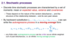
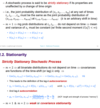
- Theta helps us decide whether the process is stationary or not (for an autoregressive process)
What are the properties of stochastic processes and how can we re-write an AR process?
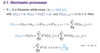
What is the expected value and variance of a stochastic/AR process?
- WE assume the distribution of the error-term –> To give us the gaussian properties
- Expected value
- As the expected value of all error terms is 0, the expected value of x is 0
- Variances
- Dont include the E(X) term as it is 0
- Variance second term –> covariance of two error terms is zero
- as σE2 is a constant we can take it outside the summation. As theta is between -1 and 1 the sum will converge. So we can use the sum of an infinite series to get (a/1-θ2) where a is the constant of theta (which is 1)
- Giving us the answer we have
- Why do we get θ2 on the bottom–>
- infinite sum series is –>(1/1-ratio) where ratio is θ2(i+1)/θ2i which leads you to θ2
- Expected value
What is the Covariance of a stochastic/AR process?
- Cov(x,y) = E(XY) - E(X)E(Y)
- As E(xt) for all value of t is 0, we just look at the expected value of E(xt,xt-1)
- We are left with only the squares as the expected value of any cross products of the error is equal to 0
- Dividing through by theta in the 4th line gives use the equation for the covariance between x and its most recent past value.

What are the special notations we need to remember about stochastic/AR processes?

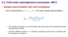
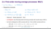
Example of first-order autoregression processes?
- These are the Autocorrelation (AC) functions
- Each step i, is 0.7i

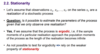
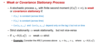
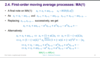
What is a general definition of Stationarity?
- Not possible to test for ergodicity
- Cant wait 1000 - infinite years to test it –>have to rely on weaker properties of stationarity
- imagine it like the number of observations in a sample
- as with CLT you need a large sample set to determine processes moments but in the case of time series data we are limited by the dimension of time
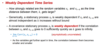
What is a Strictly Stationary Stochastic process?
DIFFERENCE BETWEEN STRICTLY AND WEAKLY STATIONARY –> this bottom part is weakly stationary??
- Think of time like an infinitely long lock and at each point of time there is an infinitely long combination of outcomes but only one realised over time
- m –> moment
- Covariances are a function of the time-shift or lag k only
- so the distance between two points (or lock digits) can affect the covariance of each realisation but that is NOT affected by starting at a future time but with the same distance between two points.
- ACF –> the length and strength of the processes ‘memory’
What is Weak or Covariance Stationary Processes?
- If the error term follows a normal distribution we can say that weak stationarity is equivalent to strict stationarity
- None of the moments depend on time!
What is a weakly dependent time series?
What is the Wold Decomposition?
- Mu = deterministic and psi = stochastic

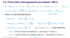
How can we represent a first-order autoregressive process AR(1)?
- (1-θL)-1
- We know that 1/1-R where R is a ratio that corresponds to the sum of a geometric series
- That is why we can convert it into 1 + θL + θ2L2….
*
How do you calculate the Sample autocorrelation coefficient?
- Still, the sample covariance divided by the sample variance
*
What are partial autocorrelations?
- can find the autocorrelation between xt and some lag k of xt without losing the effect of all lags in the middle
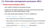
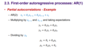
Example of generating Partial Autocorrelations?
- Gamma = Autocovariances
- Gamma(0) –> Variance
- rho –> auto correlations
- theta –> partial auto correlation?
What are the Yule-Walker Equations?
- MM –> Method of moments

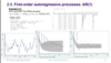
Examples of ACF and PACF?
-
inside confidence bands –> cannot reject the null the autocorrelations are equally to 0 - rewrite this
- AR(2)
- Exponential decay in ACF
PACF 2 significant PAC
- Exponential decay in ACF
- AR(2)
Example of estimating PAC from Yule-Walker equations
- End numbers are different as PAC accounts for lag effect

What is the Q-statistics for Partial Autocorrelations?

What does a MA(1) process look like and what are its respective moments?
- V(X) –> end up with the sum of the variances and the covariances of any white noise is 0
- MA series is stationary because E(X),V(X) and covariance don’t depend on time
- Weakly dependent –> autocorrelation of order 1 is different to zero, but quickly moves to 0 after the first lag so yes it is!
What do the Yule-Walker equations look like for MA(1) processes?
- First-order MA –> have partial autocorrelation that do no cut off as fast as AR(1) processes, but their AUTOCORRELATION cut off
- AC cuts off at the point of identification of the order of the equations

Example of MA Process?
- AC cuts off after 1 lag
- +VE coefficient on the lag of error
- Oscillating PAC
- -VE coefficient on lag of error
- Exponential decline in PAC

How do you move from a MA(1) to an infinite autoregressive process?
What is the general formula and characteristics of an AR(p)?
- Theta being between -1 and 1 is no longer the stationarity condition –> need to look at the roots of the characteristic equation
- Either the roots are less than 1 in absolute value or the solution to the characteristic equals are all greater than 1 in absolute value

What is the general formula and characteristics of an MA(q)?
- moving average function is always stationary by definition
- E(X), VAR(X) and COV(X) are all not a function of time?
- complex roots work the same was as AR roots
Examples of AR(p) and MA(q) correlograms?
- AR(2)
- AC ==> exponential decrease
- PAC ==> two clear PACs that are statistically significant
- MA(2)
- Ac ==> 2 statistically clear autocorrelations
- PAC ==> smooth decease in oscillating function

Example of using the characteristic and invertibility conditions for AR(p) and MA(q) processes?
- statiationarity condition for finding roots of AR(p)
- sub in for L
- get it into the form L - solutions for each bracket –> as the equation needs to equal zero
- rearrange until we get it into the characteristic equation form –> coefficient on L will therefore be the roots
- EQUALLY, YOU CAN JUST SUB IN FOR L AND FIND THE SOLUTION WHICH IS A HELL OF A LOT EASIER!
- sub in for L
- MA(q) process is always stationary so just need to check if we can invert it into an infinite order auto regressive process

Example of MA(2) process with real and complex roots?
- Complex root
- AC ==> 2 significant autocorrelations (MA(2))
- PAC ==> Smooth decrease in PAC (potentially a sine wave that’s oscillating) –> MA(2)
- Real roots
- AC ==> two significant autocorrelations
- PAC ==> smooth exponential decrease in the lags

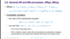
What is the equations and characteristics of an ARMA(1,1) process?
- can change to an MA(∞) process by isolating xt on one side
- Can only do this if theta is lower than one in absolute value
- if invertible we can create an AR(∞) process by isolating the error term εt on one side
- For each case, they can be converted to an infinite sum of a geometric series in a similar way to before (watch out for the coefficients!!)
- Although MA processes are always stationary we cannot able this directly to ARMA processes due to the AR component

Example of an ARMA(1,1) and AR(1) process correlograms?
Not always clear what the ARMA process will be
- ARMA(1,1)
- AC ==> sharp decrease after 1st autocorrelation then smooth decline (AR(1))?
- PAC ==> substantial decrease from 1st PAC to 2nd and 3rd but decreases in an oscillating sine wave shape similar to a MA process (MA(1))
- AR(1)
- AC ==> smooth decrease in the ACF
- PAC ==> sharp cut off after first PAC

What are the equations and characteristics of an ARMA(p,q) process?
- characteristic equation
- Get all the x’s on one side and the errors on the other ==> just like you would for for AR(p) and MA(q) processes

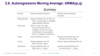
Summary of the rules we can use to identify the data generating process from is ACF and PACF?
What happens to the ARMA(p,q) process if its mean is not assumed to be 0?
- still deal with the process in the same fashion as we would have done before
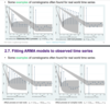
Examples of correlograms from real-world time series?
When fitting an ARMA to data we try to match the sample correlogram to the correlogram of a known theoretical ARMA process –> important part of the estimation process of the Box -Jenkins approach
- AR(1)
- AC ==> exponential decline
- PAC ==> 1 significant
- Unit Root
- AC ==> small decrease/ linear decline in AR
- PAC ==> 1 significant
- AR(2) w/ real roots
- AC ==> slow decline of ACF
- PAC ==> 2 significant
- AR(2) 2/ complex roots
- AC ==> gradual decline in ACF but as a sine wave
- PAC ==> 2 significant
What else can we use alongside the Box-Jenkins approach to help us decide on the specification of the data generation process?
- Always pick the specification that returns the lowest AIC and BIC
- Then pick the one that is the most parsimonious (with preference to the model selected under the BIC criterion)

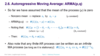
What does an impulse response look like for an ARMA process?
- Can understand the impulse response of a shock in the error term for a AR(1) process if we transform it into an infinite MA process
- IS the opposite for an MA process?
- after the first shock the value of xt is just the value of pt
- The left graph shows how the impact on x decays overtime but the right one shows how the affect accumulate on each other

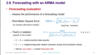
How can we forecast one period ahead with AR(I)MA processes?

How can we forecast k periods ahead with AR(I)MA processes?
- Variance is higher for the k periods model over the one period one as it is obviously harder to accurately forecast a value in 10 years rather than just one year
- From the variance, we can calculate confidence intervals for our predicted variable (where see = standard error = standard deviation).

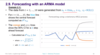
Example of forecasting using an AR(1) process?
- blue line is calculated from the last know x value we have in our sample
How can we assess the performance of a forecasting model?
What are the different types of forecasts we can do?
- Static ==> input the most recent value observed (usually used for one period)
- Dynamic ==> use our forecasted values to predict future values
