Hypothesis Testing

Question 1

what is statistical inference?

Answer 1

—Making decisions in the face of uncertainty. making decisions on the basis that the result achieved was not due to chance or random process
—Hypothesis testing is a structure for making these decisions

Question 2

What are two types of hypothesis?

Answer 2

The null hypothesis and alternative hypothesis

Question 3

distinguish between type 1 and type 2 error when might they occur?

Answer 3

Type 1 error: rejecting null hypothesis despite it being true. probability of type 1 error occuring is level of significant α

Type 2 error: retain null hypothesis when it is false/ probability of type 2 error occuring is β

these errors might occur during the process of hypothesis testing

Question 4

what does hypothesis testing consist of?

Answer 4

statement of null hypothesis and selecting significance level. then acquiring data through calculation

statistical calculations tell us whether to reject null hypothesis or not

Question 5

how is alpha related to type 1 error?

Answer 5

value of alpha, which is related to the level of significance that we selected has a direct bearing on type I errors. Alpha is the maximum probability that we have a type I error. For a 95% confidence level, the value of alpha is 0.05. This means that there is a 5% probability that we will reject a true null hypothesis. In the long run, one out of every twenty hypothesis tests that we perform at this level will result in a type I error.

Reduce alpha to reduce chance of type 1 error

Question 6

what happens when we decrease probability of an error from occuring?

Answer 6

e probability for the other type increases. We could decrease the value of alpha from 0.05 to 0.01, corresponding to a 99% level of confidence. However, if everything else remains the same, then the probability of a type II error will nearly always increase.

Question 7

what does the alpha level suggest?

Answer 7

95% Certainty of making the right decision”

Question 8

what is the conventional alpha level?

Answer 8

—Convention: set level of type 1 error (α) to 5% (i.e. 5% chance we reject H0 when it is true), ignore type 2 error (β).

Question 9

when we start a hypothesis, what do we first assume?

Answer 9

—assuming null is true. Then, gather data, and if we are faced with enough evidence, we will switch from null to alternative hypothesis.

Question 10

features of null and alternative hypothesis

Answer 10

—Null hypothesis:
—Always about a population value (greek letter)
—Always has an “=“
—
—
—Alternative hypothesis:
—Always about a population value (greek letter)
—Has one of <, > or ≠
—Looks like null, but “=“ has been replaced.

Question 11

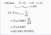
—A store manager is considering a new billing system for credit customers. New system will only be cost effective if mean monthly account is more than $170. Random sample of 400 monthly accounts gives sample average of $178. Manager knows that accounts are approximately normally distributed, with standard deviation of $65.
—Can the manager conclude from this data that the new system will be cost effective?
—Want to find out if µ, true mean monthly account, is bigger than $170.

Answer 11

Null hypothesis

H0:µ=170

—Alternative hypothesis

HA:µ>170

Question 12

what does central limit theorem suggest in regards to hypothesis testing?

Answer 12

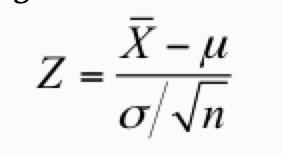
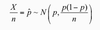
—Says that sample average has a normal distribution, centre at µ, standard deviation of σ/√n.—So, if we calculate ( X̄ - µ)/ ( σ / √n) it should follow a standard normal distribution.

Question 13

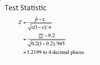
in hypothesis testing, what is a test statistic?

Answer 13

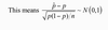
—We calculate a test statistic – this measures (in standardised units) how far from the hypothesised µ our sample average is

—Z should follow a standard normal distribution IF the true µ is equal to the one in our null hypothesis.

Question 14

list the two methods in the decision rule

Answer 14

Rejection region

p-value

Question 15

Decision rule

-rejection region

Answer 15

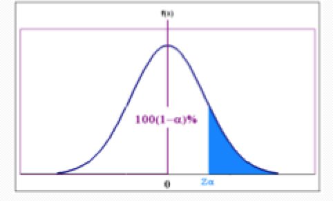
—Say we want to be 95% certain. This means a 5% chance of rejecting H0 when it is true.
So, we find the EXTREME 5% of the standard normal (according to our alternative hypothesis) and this will be our rejection region

Question 16

if test statistic is 2.46, describe what to do

Answer 16

—Point that marks off top 5% of a standard normal is 1.645.
—So, we will reject the null hypothesis if our test statistics lies above 1.645.
—Here, Test statistic = 2.46.

—Reject the null hypothesis. There is sufficient evidence to conclude that the mean monthly bill is higher than $170.

Question 17

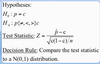
4 steps for hypothesis test

Answer 17

1. Null and alternative hypotheses
2. Test statistic
3. Decision Rule: Rejection Region or p-value – found from appropriate distribution (std normal)
4. Conclusion

Question 18

Decision rule

describe the p-value

Answer 18

—This is probability of getting our test statistic equal or more extreme than the sample result, given that null hypothesis is true

also known as observed level of significane

Question 19

how to use p-value in making decision of whether to reject null hypothesis

Answer 19

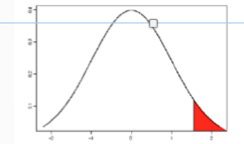
—Draw a diagram – it is the area more extreme than our test statistic, i.e. for the last example, p-value is P(Z>2.46).
—Small p-value is evidence against the null hypothesis. For 5% chance of error, we set small to be
—if p-value is smaller than α, then we will reject null hypothesis; get same conclusion from p-value and rejection region methods.

If p value is greater than or equal to α, do not reject null hypothesis

Question 20

Describe one tailed test

Answer 20

—If the alternative hypothesis is “”
—This is a one tailed test
—Rejection region will be in either upper or lower tail
—P-value is the probability of getting a more extreme result

Question 21

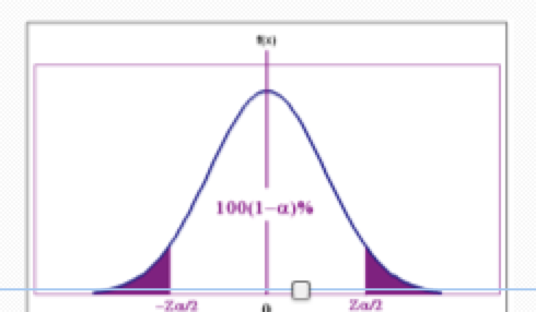
describe two tailed test

Answer 21

—If the alternative hypothesis is “≠”
—This is a two tailed test
—Rejection region needs to be split between both tails
—P-value will include an absolute value – i.e. will be the probability of getting further away from the hypothesised mean on either side

Question 22

if alternative is “≠“

Answer 22

—Rejection Region will be Z+Zα/2
—P-value will be P(Z>|T.S|)+P(Z

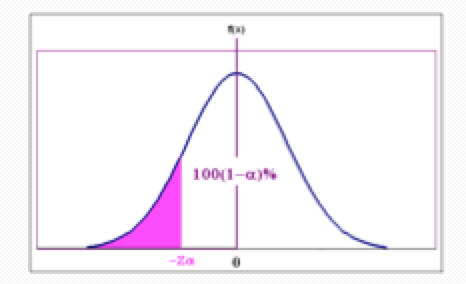
Question 23

If alternative is “

Answer 23

—Left tailed test
—Rejection Region will be Z
—P-value will be P(Z

Question 24

So if alternative is “>“

Answer 24

—Right tailed test
—Rejection Region will be Z>+Zα
—P-value will be P(Z>T.S)

Question 25

—A new drug to treat headaches has been developed, but its effectiveness is very sensitive to dosage – too much and side effects occur, whilst if too little is given then the headache may remain.
A pharmaceutical company are manufacturing the drug in tablets, and claiming they contain on average 100mg of the active ingredient. A sample of 25 tablets gives an average of 106 mg. Assuming that the standard deviation of active ingredient content is 13mg, determine if the company’s claim is supported by the data

Answer 25

—Let the active ingredient content of a single tablet be denoted by X, where X is in mg.
X̄ = 106 n =25 standard deviation = 13
—Want to test if μ=100 or not (i.e. a two sided test).

<!--StartFragment-->

Step 1: Hypotheses<!--EndFragment-->

H0: μ = 100

H_A: μ ≠ 100

Step 2: Test statistic

Z= X̄ - μ/ σ/ √n = 106-100/ 13/5= 2.308 (3dp)

<!--StartFragment-->

Step 3: Decision Rule<!--EndFragment-->

—P-value = probability of getting this value of the test statistic or “less common” if the null hypothesis is true
—Calculated as the region in the tails
—P-value = P(Z>2.308)+P(Z

                                                         = 2\* P(Z

                                                           ≈ 2\* P(Z

= 2* 0.0104

= 0.0208

<!--StartFragment-->

Conclusion<!--EndFragment-->

—Here, the probability of getting this test statistic (getting this data) if the null hypothesis is true is 0.0208.
—This is small (smaller than a significance level of 5%).
—Hence we reject the null hypothesis. The evidence casts doubt on the company’s claim of 100mg average in each tablet.

Question 26

what does the test statistic measure?

Answer 26

This measures how far our sample value is from the hypothesised value in “standardised units”

Question 27

Does CLT apply to proportions?

Answer 27

applies to sample proportions, if the sample is large enough

Question 28

—The sample proportion has a normal distribution, with a centre at p, the population proportion, and variance of
P(1-p)/n

what does this mean?

Answer 28

Question 29

how does sample proportion relate to hypothesis testing?

Answer 29

—we use the test value of p (i.e. the value in the null hypothesis) for calculating the standard error.

Question 30

—In the data set about use of a cycle way along a river (discussed in Section 6 part b), 204 of the 945 people are found to be walking.
—It is supposed that overall, 20% of users are walkers. Test this supposition using the data.

Answer 30

H_o: p= 0.2

HA : P ≠ 0.2

—Rejection Region: For 5% significance, two tailed test, reject H₀ if test statistic is less than -1.96 or greater than +1.96.

OR

—P-value= P(|Z|>1.2199)=2*P(Z>1.22)
=2*[0.5-P(0

=0.2224

—As the test statistic does not lie in the rejection region, we do not reject the null hypothesis. The data do not disagree with the claimed proportion of walkers.

OR

—As the p-value is large (0.224>α=0.05), we do not reject the null hypothesis. The data do not disagree with the claimed proportion of walkers.

Question 31

If we are interested in the population mean, then

Answer 31

—we can find confidence intervals and perform hypothesis tests, IF we know the population standard deviation

Question 32

<!--StartFragment-->

What if we don’t know σ (population standard deviation)?

Answer 32

we cannot substitute *s *in for σ since (x̄ - μ)/ ( s/ √n ) does not have standard normal distribution

it does follow known distribution (x̄ - μ)/ ( s/ √n ) follows a t-distribution with n-1 degrees of freedom

Question 33

about t distribution

Answer 33

• —It is symmetric around 0

bell shaped (like a normal)

• t distribtion has more area in tails and less in the centre than does the standardized normal distribution (S is used to estimate the unknown σ, values ot t more variable than those for Z)
• —The higher the degrees of freedom, the more normal the curve looks.
• Mean and median= 0

Question 34

what happens when degrees of freedom and sample size increase?

Answer 34

S becomes better estimate of σ, t distribution gradually approaches standardized normal distribution until two are identical

eg. sample size of 120 or more, S esimates σ closely enough, litle difference between t and Z distributions

Question 35

describe difference between t distribution in theory and in practice

Answer 35

theory: t distribution assumes random variable X is normally distributed
practice: sample size large enough, population not very skewed, use t distribution to estimate the population mean when σ is unknown

Question 36

what happens when there is a small sample size and skewed population distribution?

Answer 36

confidence interval may not provide valid estimation of the population mean

Question 37

how to assess assumption of normality?

Answer 37

evaluate sape of sample data by creating

• histogram
• stem and leaf display
• boxplot
• normal probability plot
• these graphs have limited application when sample size is small

Question 38

when there is 95% confidence level, this means that there is

Answer 38

2.5% of the values (area of 0.025) in each tail of the distribution

cumulative probabilty of 0.975

upper tail value is +1.9842

lower tail value is -1.9842

Question 39

what is the test statistic for hypothesis testing?

Answer 39

T = X̄- μ/ s/ √n

Question 40

—A report produced for a local area government claims that over a particular suburb when planes are overhead the mean noise level is no more than 60dB. A group of residents in the suburb conduct a test, measuring noise levels on 18 occasions when planes are overhead and obtain an average of 72dB with a standard deviation of 10dB.
—Does the resident’s data cast doubt on the government claim?

Answer 40

—H0: µ=60
—HA: µ>60

T = X̄- μ/ s/ √n = 72-60/ 10/√18 = 5.091

<!--StartFragment-->

Rejection Region<!--EndFragment-->

—Need to compare to t distribution with 17 degrees of freedom.
—See Table 3 in text
—Go to row marked for DF=17.
—Want a one tailed test.
—For 5% error, want to find upper 5%.
—Value is 1.7396. Rejection region is t>1.7396.

—Since our test statistic lies within the rejection region, (5.091>1.7396) we reject the null hypothesis. The resident’s data casts doubt on the government’s claim.

Question 41

bottom row that has df=∞, what should you do?

Answer 41

—this is the standard normal probabilities.
—If df is very large, use Z tables even if σ is unknown

—If df is not on tables as exact, use whatever df is closest
—Difference between values for large df is small
E.g. df=114; would use values for df=110 as this is closest.

Question 42

—You are accepting delivery of a shipment of synthetic diamonds, whose average weight is supposed to be 0.5 carats (or more).
—You quickly take a random sample of 6 stones and find the following weights:

0.46, 0.51, 0.52, 0.48, 0.47, 0.54.

—You are suspicious that the true mean weight is less than 0.5 carats. Do you have enough evidence to conclude that the mean weight in the shipment is less than 0.5 carats? Use a 5% significance level, and assume that the stones’ weights follow a normal distribution.

Answer 42

—Default position: shipment really does have average weight over 0.5 carats; simple null

H0: µ=0.5

HA: µ

T=X̄- μ₀/ s/ √n

—Compare to t-distribution with n-1=5df.
—From tables, P(t₅>0.7267)=P(t₅
—So, P(t₅0.25.
—Note: we cannot get a p-value from tables for a t-test; above we can find that the p-value is larger than 0.25, but cannot get the value exactly. We need Minitab to get a p-value for a t-test, as below.
—
—From Minitab, P(t5

—Test statistic does not lie in rejection region (by hand); p-value is large (>40% from Minitab).
Hence we do not reject the null hypothesis. Insufficient evidence to claim the average is smaller than 0.5

Question 43

when else may you use t distribution?

Answer 43

—use t-distribution for confidence intervals for µ when σ is unknown.

—σ has been estimated from data, confidence interval (always two tailed) will be of form

Question 44

—Find a 99% confidence interval for the population mean noise level given the resident’s data (that is, from a sample of size 18, an average of 72dB and standard deviation of 10dB).

Answer 44

Question 45

If μ0 lies in the 95% CI based on the observed data

Answer 45

we would accept H0 in testing μ= μ0 vs a two-sided alternative at the 5% significance level.

Question 46

when you fail to reject the null hypothesis, what can you conclude?

Answer 46

there is insufficient evidence to warrant its rejection

Question 47

what is the critical value?

Answer 47

the critical value divides the rejection region from the non-rejection region

Question 48

what is the confidence coefficient?

Answer 48

probability that you will not reject the null hypothesis H_owhen it is true and should not be rejected

Complement of Type 1 error (1-α)

Question 49

what is the power of a statisical test?

Answer 49

probabilty that you wil reject the null hypothesis when it is false and should be rejected

Question 50

what is a way to reduce type 2 error?

Answer 50

by increasing sample size so that there will be smaller difference between hypothesized values and actual population parameters

Question 51

describe connection between confidence interval estimation and hypothesis testing

Answer 51

if hypothesised value is contained within the interval, you do not reject the null hypothesis

it if is outside interval, you reject null hypothesis