Statistics Flashcards
(129 cards)
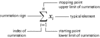
population
set of all individuals of interest in a study population = parameter
parameter
numerical value that describes a population can be a single measurement or set of measurements
sample
set of individuals selected from a population, representative of population in a study sample = statistic
statistics
numerical value that describes a sample can be a single measurement or set of measurements
descriptive statistic
statistical procedures that are used to summarize, organize, simplify data - make raw score meaningful e.g. mean, median, mode
inferential statistics
techniques that allow us to study samples then make generalizations about the population - infer sample -> population
sampling error
discrepancy/ amount of error that exists between a sample statistic and population parameter - important to consider in inferential statistics
construct
internal attributes/ characteristics that cannot be directly observed but are useful for describing and explaining behavior - hypothetical e.g happiness
operational definition
defines construct in terms of observable behaviors e.g. intelligence defines as performance on IQ test
nominal scale
categorical organization - can only measure qualitative difference e.g gender, country of origin, hair color
ordinal scale
categories organized in a certain sequence, differences are quantitative - amount between one person and next is not consistent e.g. class rank, rating scale
interval scale
ordered categories that are intervals of exactly same size with an arbitrary zero point - 0 does not mean the absence of the construct being measured e.g. celsius scale, temp
ratio scale
interval scale with absolute zero point - can describe differences between categories in terms of ratios (one thing is 3 times larger than another) e.g. weight, height, speed
discrete variables
separate, indivisible categories - whole numbers or specific categories - no decimals e.g 3 goals scores
continuous variables
infinite number of possible values that fall between any two observed values - divisible into infinite number of fractional parts e.g. height
real limits
boundaries of intervals for scores that are represented on a continuous number line - each score has two limits, half way between scores (upper real limit, lower real limit) e.g. if you have observed value of 8, actually represents range from 7.5 - 8.5 (kind of like rounding)
correlational method
two variables observed to see if there is a relationship between the two
experimental method
establishes cause and effect relationship between variables - must manipulate one variable, observe second - controlled research situation
non-experimental method
variable determines group (those that have depression) - don’t manipulate
independent variable
manipulated variable - 2+ treatment conditions
dependent variable
observed for changes to assess effect
control
does not receive manipulated experimental treatment, baseline for comparison
quasi-independent variable
groups not created by manipulating independent variable - participent variable (male/female) - time variable (before/after)
summation notation
a way to represent scores n ∑ xi i = 1 i = the starting point of the scores n = the stopping point