Define the basic indicator approach, the standardized approach, and the alternative standardized approach for calculating the operational risk capital charge
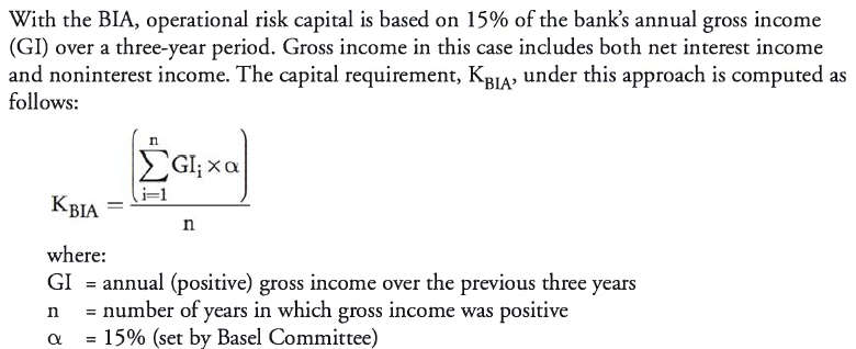
Basel II proposed three approaches for determining the operational risk capital requirement (i.e., the amount of capital needed to protect against the possibility of operational risk losses). The basic indicator approach (BIA) and the standardized approach (TSA) determine capital requirements as a multiple of gross income at either the business line or institutional level. The advanced measurement approach (AMA) offers institutions the possibility to lower capital requirements in exchange for investing in risk assessment and management technologies.
Basic Indicator Approach
The BIA for risk capital is simple to adopt, but it is an unreliable indication of the true capital needs of a firm because it uses only revenue as a driver. For example, if two firms had the same annual revenue over the last three years, but widely different risk controls, their capital requirements would be the same. Note also that operational risk capital requirements can be greatly affected by a single year’s extraordinary revenue when risk at the firm has not materially changed.
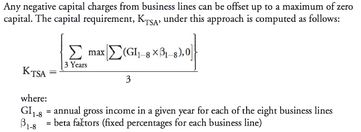
The Standardized Approach
For the standardized approach (TSA), the bank uses eight business lines with different beta factors to calculate the capital charge. With this approach, the beta factor of each business line is multiplied by the annual gross income amount over a three-year period. The results are then summed to arrive at the total operational risk capital charge under the standardized approach. The beta factors used in this approach are shown as follows:
- Investment banking (corporate finance): 18%.
- Investment banking (trading and sales): 18%.
- Retail banking: 12%.
- Commercial banking: 13%.
- Settlement and payment services: 18%.
- Agency and custody services: 15%.
- Asset management: 12%.
- Retail brokerage: 12%.
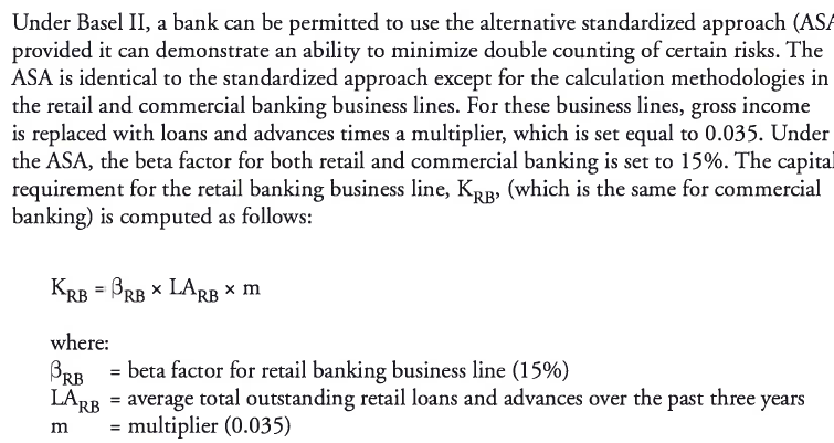
Alternative Standardized Approach
Unanticipated Results from Negative Gross Income
The BIA and TSA capital charge methodologies can produce inappropriate results when accounting for negative gross income.
The Basel Committee has recognized that capital under Pillar 1 (minimum capital requirements) may be distorted and, therefore, recommends that additional capital should be added under Pillar 2 (supervisory review) if negative gross income leads to unanticipated results.
Describe the modeling requirements for a bank to use the Advanced
Measurement Approach (AMA)
The advanced measurement approach (AMA) allows banks to construct their own models for calculating operational risk capital. Although the Basel Committee allows significant flexibility in the use of the AMA, there are three main requirements. A bank must:
- Demonstrate an ability to capture potentially severe “fat-tail” losses (banks must use 99.9th percentile events with a one-year time horizon).
- Include internal loss data, external loss data, scenario analysis, and business environment internal control factors (i.e., the four data elements).
- Allocate capital in a way that incentivizes good behavior (i.e., create incentives to improve business line operational risk management).
Under the AMA, capital requirements should be made for all seven risk categories specified by Basel II. Some firms calculate operational risk capital at the firm level and then allocate down to the business lines, while others calculate capital at the business line level. Capital calculations are typically performed by constructing a business line/event type matrix, where capital is allocated based on loss data for each matrix cell.
Additional quantitative requirements under the AMA include:
- The approach must capture all expected and unexpected losses and may only exclude expected losses under certain criteria as stated in Basel II.
- The approach must provide sufficient detail to ensure that fat-tail events are captured.
- The bank must sum all calculated cells in the business line/event type matrix and be able to defend any correlation assumptions made in its AMA model.
- All four data elements must be included in the model, including the use of internal and external data, scenario analysis, and business environment factors.
- The bank must use appropriate weights for the four data elements when determining operational risk capital.
While the four data elements must be considered in the capital calculations, many banks use some of these elements only to allocate capital or perform stress tests, and then adjust their models, rather than using them as direct inputs into capital calculations. Regulators have accepted many different types of AMA models, such as the loss distribution approach, given the rapid development of modeling operational risk capital.
Describe the loss distribution approach to modeling operational risk
capital
The loss distribution approach (LDA) relies on internal losses as the basis of its design. A simple LDA model uses internal losses as direct inputs with the remaining three data elements being used for stressing or allocation purposes. However, according to Basel II, a bank must have at least five years of internal loss data regardless of its model design but can use three years of data when it first moves to the AMA.
- The advantage of the LDA is that it is based on historical data relevant to the firm.
- The disadvantage is that the data collection period is likely to be relatively short and may not capture fat-tail events. For example, no firm can produce 1,000 years of data, but the model is supposed to provide a 99.9% confidence level.
- Also, some firms find that they have insufficient loss data to build a model, even if they have more than five years of data.
- Additionally, banks need to keep in mind that historical data is not necessarily reflective of the future because firms change products, processes, and controls over time.
Explain how frequency and severity distributions of operational losses are obtained, including commonly used distributions and suitability guidelines for probability distributions
Modeling Frequency
- When developing a model of expected operational risk losses, the first step is to determine the likely frequency of events on an annual basis. The most common distribution for modeling frequency is the Poisson distribution. This distribution uses only one parameter, λ, which represents the average number of events in a given year, as well as the distribution’s mean and variance. In an LDA model, λ can be obtained by observing the historical number of internal loss events per year and then calculating the average.
- The Poisson distribution represents the probability of a certain number of events occurring in a single year.
Modeling Severity
- The next step in modeling expected operational risk losses is to determine the likely size (i.e., severity) of an event. The most common and least complex approach is to use a lognormal distribution. However, low frequency losses may be a better fit to distributions such as Generalized Gamma, Transformed Beta, Generalized Pareto, or Weibull. Regulators are interested in the selected distribution’s “goodness of fit.”
Explain how Monte Carlo simulation can be used to generate additional data points to estimate the 99.9th percentile of an operational loss distribution
Once the frequency and severity distributions have been established, the next step is to combine them to generate data points that better estimate the capital required. This is done to ensure that likely losses for the next year will be covered at the 99.9% confidence level. Monte Carlo simulation can be used to combine frequency and severity distributions (a process known as convolution) in order to produce additional data points with the same characteristics as the observed data points.
With this process, we make random draws from the loss frequency data and then draw those events from the loss severity data. Each combination of frequency and severity becomes a potential loss event in our loss distribution.
Explain the use of scenario analysis and the hybrid approach in modeling operational risk capital
- Scenario analysis data is designed to identify fat-tail events, which is useful when calculating the appropriate amount of operational risk capital. The advantage of using scenario analysis is that data reflects the future through a process designed to consider “what if” scenarios, in contrast to the LDA which only considers the past. The major disadvantage of scenario analysis is that the data is highly subjective, and it only produces a few data points. As a result, complex techniques must be applied to model the full loss distribution, as the lack of data output in scenario analysis can make the fitting of distributions difficult. In addition, small changes in assumptions can lead to widely different results.
- While some scenario-based models have been approved in Europe, U.S. regulators generally do not accept them.
- In the hybrid approach, loss data and scenario analysis output are both used to calculate operational risk capital. Some firms combine the LDA and scenario analysis by stitching together two distributions. For example, the LDA may be used to model expected losses, and scenario analysis may be used to model unexpected losses. Another approach combines scenario analysis data points with actual loss data when developing frequency and severity distributions.
Insurance and its influence on operating risks
A bank using the AMA for calculating operational risk capital requirements can use insurance to reduce its capital charge. However, the recognition of insurance mitigation is limited to 20% of the total operational risk capital required.
Insurance typically lowers the severity but not the frequency.
Standardized measurement approach (SMA)
The standardized measurement approach (SMA) represents the combination of a financial statement operational risk exposure proxy (termed the business indicator, or BI) and operational loss data specific for an individual bank. Because using only a financial statement proxy such as the BI would not fully account for the often significant differences in risk profiles between medium to large banks, the historical loss component was added to the SMA to account for future operational risk loss exposure.
The Business Indicator
The business indicator (BI) incorporates most of the same income statement components that are found in the calculation of gross income (GI). A few differences include:
- Positive values are used in the BI (versus some components incorporating negative values into the GI).
- The BI includes some items that tie to operational risk but are netted or omitted from the GI calculation.
The SMA calculation has evolved over time, as there were several issues with the first calculation that were since remedied with the latest version. These items include:
- Modifying the service component to equal max(fee income, fee expense) + max(other operating income, other operating expense). This change still allowed banks with large service business volumes to be treated differently from banks with small service businesses, while also reducing the inherent penalty applied to banks with both high fee income and high fee expenses.
- Including dividend income in the interest component, which alleviated the differing treatment among institutions as to where dividend income is accounted for on their income statements.
- Adjusting the interest component by the ratio of the net interest margin (NIM) cap (set at 3.5%) to the actual NIM. Before this adjustment, banks with high NIMs (calculated as net interest income divided by interest-earning assets) were penalized with high regulatory capital requirements relative to their true operational risk levels.
- For banks with high fee components (those with shares of fees in excess of 50% of the unadjusted BI), modifying the BI such that only 10% of the fees in excess of the unadjusted BI are counted.
- Netting and incorporating all financial and operating lease income and expenses into the interest component as an absolute value to alleviate inconsistent treatment of leases.
Business Indicator Calculation
The BI is calculated as the most recent three-year average for each of the following three components:
BI = ILDCavg + SCavg + FCavg
where:
- ILDC = interest, lease, dividend component
- SC = services component
- FC = financial component
The three individual components are calculated as follows, using three years of average data:
interest, lease, dividend component (ILDC) =
min[abs(IIavg - IEavg), 0.035 x IEAavg] + abs(LIavg - LEavg) + DIavg
where:
- abs = absolute value
- II = interest income (excluding operating and finance leases)
- IE = interest expenses (excluding operating and finance leases)
- IEA = interest-earning assets
- LI = lease income
- LE = lease expenses
- DI = dividend income
services component (SC) =
max(OOIavg, OOEavg) + max{abs(FIavg - FEavg), min[max(FIavg, FEavg), 0.5 x uBI + 0.1 x (max(FIavg, FEavg) - 0.5 x uBI)]}
where:
- OOI = other operating income
- OOE = other operating expenses
- FI = fee income
- FE = fee expenses
- uBI = unadjusted business indicator = ILDCavg + max(OOIavg, OOEavg) + max(FIavg, FEavg) + FCavg
financial component (FC) = abs(net P<Bavg ) + abs(net P&LBBavg)
where:
- P&L = profit & loss statement line item
- TB = trading book
- BB = banking book
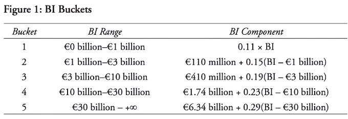
For the purposes of calculating the SMA, banks (based on their size for the BI component) are divided into five buckets as shown in Figure 1.
The BI component calculation should exclude all of the following P&L items:
- administrative expenses,
- recovery of administrative expenses,
- impairments and impairment
- reversals, provisions and reversals of provisions (unless they relate to operational loss events),
- fixed asset and premises expenses (unless they relate to operational loss events),
- depreciation and amortization of assets (unless it relates to operating lease assets),
- expenses tied to share capital repayable on demand,
- income/expenses from insurance or reinsurance businesses,
- premiums paid and reimbursements/payments received from insurance or reinsurance policies,
- goodwill changes, and corporate income tax.
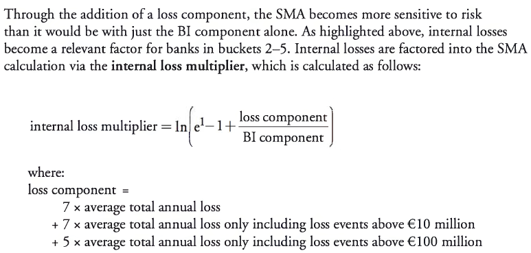
Internal Loss Multiplier Calculation
Ideally, a bank will have 10 years of quality data to calculate the averages that go into the loss component calculation. If 10 years are not available, then during the transition to the SMA calculation, banks may use 5 years and add more years as time progresses until they reach the 10-year requirement. If a bank does not have 5 years of data, then the BI component becomes the only component of the SMA calculation.
- A bank whose exposure is considered average relative to its industry will have a loss component equivalent to its BI component; this implies an internal loss multiplier equal to one and an SMA capital requirement equal to its BI component.
- If a bank’s loss experience is greater (less) than the industry average, its loss component will be above (below) the BI component and its SMA capital will be above (below) the BI component.
SMA Capital Requirement Calculation
The SMA is used to determine the operational risk capital requirement and is calculated as follows:
For BI bucket 1 banks:
SMA capital = BI component
For BI bucket 2—5 banks:
SMA capital = 110M + (BI component - 110M) x internal loss multiplier
For banks that are part of a consolidated entity, the SMA calculations will incorporate fully consolidated BI amounts (netting all intragroup income and expenses). At a subconsolidated level, the SMA uses BI amounts for the banks that are consolidated at that particular level. At the subsidiary level, the SMA calculations will use the BI amounts from the specific subsidiary. If the BI amounts for a subsidiary or subconsolidated level reach the bucket 2 level, the banks must incorporate their own loss experiences (not those of other members of the group). If a subsidiary of a bank in buckets 2—5 does not meet the qualitative standards associated with using the loss component, the SMA capital requirement is calculated using 100% of the BI component.
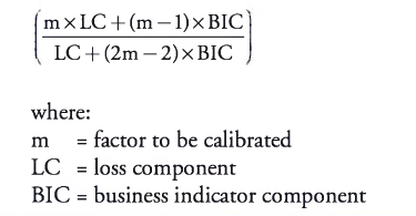
It is possible that the Committee will consider an alternative to the calculation of the internal loss multiplier shown earlier, which would replace the logarithmic function with a maximum multiple for the loss component. The formula for the internal loss multiplier would then be updated as:
Compare the SMA to earlier methods of calculating operational risk capital, including the Alternative Measurement Approaches (AMA), and explain the rationale for the proposal to replace them.
The advanced measurement approach, which was introduced as part of the Basel II framework in 2006, allowed for the estimation of regulatory capital based on a range of internal modeling practices. This approach was a principles-based framework allowing for significant flexibility. Although the hope of the Basel Committee was for best practices to emerge as flexibility declined, this never happened and challenges associated with comparability among banks (due to a wide range of modeling practices) and overly complex calculations remained.
Given these challenges, the Basel Committee set a goal of creating a new measure to allow for greater comparability and less complexity relative to prior methods. The SMA was created as this measure, with the intent of providing a means of assessing operational risk that would include both a standardized measure of operational risk and bank-specific loss data. Unlike AMA, the SMA is a single, non-model-based method used to estimate operational risk capital that combines financial statement information with the internal loss experience of a specific bank. The SMA is to be applied to internationally active banks on a consolidated basis, whereas it is optional for non-internationally active institutions. Although it is a relatively new measure, the SMA combines key elements of the standardized approach along with an internal loss experience component that was central to older approaches.
Describe general criteria recommended by the Basel Committee for the identification, collection, and treatment of operational loss data.
Banks that incorporate the loss component into the SMA calculation must follow the following general criteria:
- Documented processes and procedures must be in place for the identification, collection, and treatment of internal loss data.
- A bank must maintain information on each operational risk event, including gross loss amounts, the date of occurrence (when the event first began or happened), the date of discovery (when the bank became aware of the event), the date of accounting (when the reserve, loss, or loss provision was first recognized in the bank’s income statement, any gross loss amount recoveries, and what the drivers were of the loss event itself).
- Specific criteria must exist for loss data assignments stemming from centralized function events and related events over time (considered grouped losses).
- For the purposes of calculating minimum regulatory capital per the SMA framework, operational risk losses tied to credit risk will be excluded from the calculation.
- Operational risk losses tied to market risk will be included in the SMA calculation.
- A bank has to be able to document any criteria used to allocate losses to specific event types. In addition, a bank must be able to categorize historical internal loss data into the appropriate Level 1 supervisory categories per the Basel II Accord (Annex 9) and be prepared to provide this to supervisors when requested.
- An observation period of 10 years must be used as a basis for internally generated loss data calculations. On an exception basis and as long as good-quality data is not available for more than a five-year period, a bank first moving to the SMA can use a five-year observation period.
- Internal loss data must be comprehensive in nature and capture all material exposures and activities across all geographic locations and subsystems. When a bank first moves to the SMA, a €20,000 de minimis gross loss threshold is acceptable. Afterward, this threshold is lowered to €10,000.
Describe specific criteria recommended by the Basel Committee for the identification, collection, and treatment of operational loss data.
In addition to the general criteria noted previously, specific criteria must also be followed as described as follows:
- A policy must exist for each bank that sets the criteria for when an operational risk event or loss (which is recorded in the internal loss event database) is included in the loss data set for calculating the SMA regulatory capital amount (i.e., the SMA loss data set).
- For all operational loss events, banks must be able to specifically identify gross loss amounts, insurance recoveries, and non-insurance recoveries. A gross loss is a loss before any recoveries, while a net loss takes into account the impact of recoveries. The SMA loss data cannot include losses net of insurance recoveries.
- In calculating the gross loss for the SMA loss data set, the following components must be included:
- External expenses (legal fees, advisor fees, vendor costs, etc.) directly tied to the operational risk event itself and any repair/replacement costs needed to restore the bank to the position it was in before the event occurring.
- Settlements, impairments, write-downs, and any other direct charges to the banks income statement as a result of the operational risk event.
- Any reserves or provisions tied to the potential operational loss impact and booked to the income statement.
- Losses (tied to operational risk events) that are definitive in terms of financial impact but remain as pending losses because they are in transition or suspense accounts not reflected on the income statement. Materiality will dictate whether the loss is included in the data set.
- Timing losses booked in the current financial accounting period that are material in nature and are due to events that give rise to legal risk and cross more than one financial accounting period.
- In calculating the gross loss for the SMA loss data set, the following components must be excluded.
- The total cost of improvements, upgrades, and risk assessment enhancements and initiatives that are incurred after the risk event occurs.
- Insurance premiums.
- The costs associated with general maintenance contracts on property, plant, and equipment (PP&E).
- For every reporting year of the SMA regulatory capital, the gross losses included in the loss data set must incorporate any financial adjustments (additional losses, settlements, provision changes) made within the year for risk events with reference dates up to 10 years before that reporting year. The operational loss amount after adjustments must then be identified and compared to the €10 million and €100 million threshold.
- The only two dates a bank can use to build its SMA loss data set are the date of discovery or the date of accounting. For any legal loss events, the date of accounting (which is when the legal reserve representing the probable estimated loss) is the latest date that can be used for the loss data set.
- Any losses that are related to a common operational risk event or are related by operational risk events over time are considered grouped losses and must be entered as a single loss into the SMA loss data set.
- The circumstances, data types, and methodology for grouping data should be defined with criteria found in the individual banks internal loss data policy. In instances where individual judgment is needed to apply the criteria, this must be clarified and documented.
Explain the importance and challenges of extreme values in risk management
- The challenge of analyzing and modeling extreme values is that there are only a few observations for which to build a model, and there are ranges of extreme values that have yet to occur.
- To meet the challenge, researchers must assume a certain distribution. The assumed distribution will probably not be identical to the true distribution; therefore, some degree of error will be present.
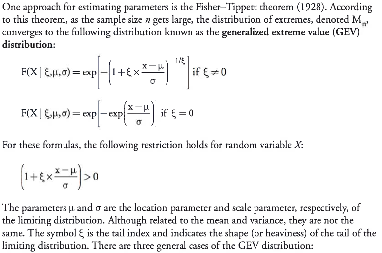
Describe extreme value theory (EVT) and its use in risk management
Extreme value theory (EVT) is a branch of applied statistics that has been developed to address problems associated with extreme outcomes. EVT focuses on the unique aspects of extreme values and is different from “central tendency” statistics, in which the central-limit theorem plays an important role. Extreme value theorems provide a template for estimating the parameters used to describe extreme movements.
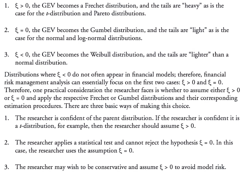
Three general cases of the GEV distribution
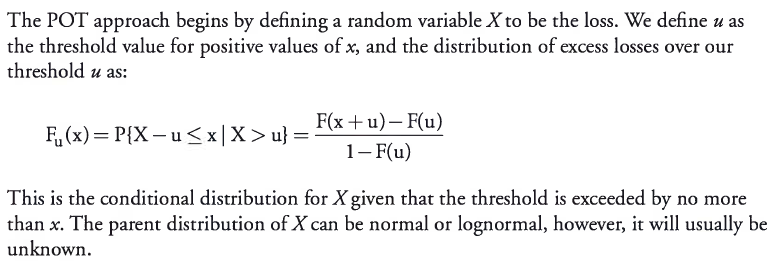
Describe the peaks-over-threshold (POT) approach
The peaks-over-threshold (POT) approach is an application of extreme value theory to the distribution of excess losses over a high threshold. The POT approach generally requires fewer parameters than approaches based on extreme value theorems. The POT approach provides the natural way to model values that are greater than a high threshold, and in this way, it corresponds to the GEV theory by modeling the maxima or minima of a large sample.
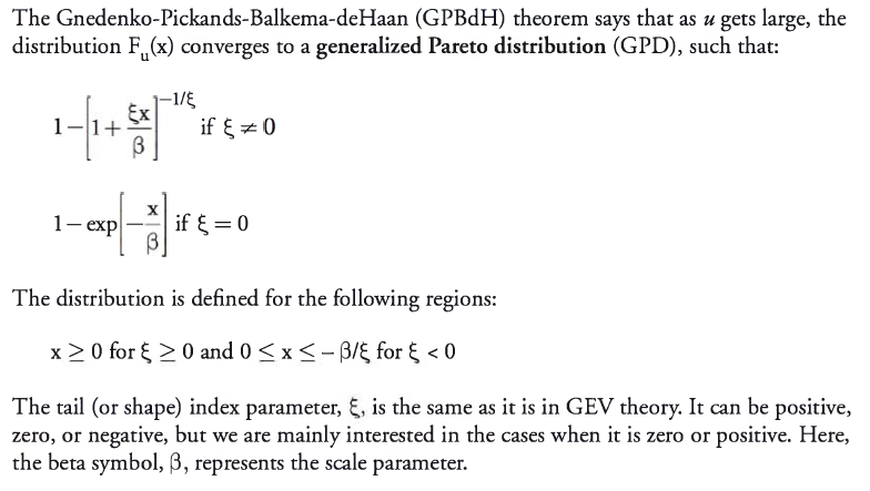
Evaluate the tradeoffs involved in setting the threshold level when applying the GP distribution
- The GPD exhibits a curve that dips below the normal distribution prior to the tail. It then moves above the normal distribution until it reaches the extreme tail. The GPD then provides a linear approximation of the tail, which more closely matches empirical data.
- Since all distributions of excess losses converge to the GPD, it is the natural model for excess losses. It requires a selection of u, which determines the number of observations, Nu, in excess of the threshold value. Choosing the threshold involves a tradeoff. It needs to be high enough so the GPBdH theory can apply, but it must be low enough so that there will be enough observations to apply estimation techniques to the parameters.

-
Topics 1-225
-
Topics 3-525
-
Topics 6-928
-
Topics 10-1217
-
Topics 13-1530
-
Topics 16-1823
-
Topics 19-2041
-
Topics 21-2334
-
Topics 24-2626
-
Topics 27-3038
-
Topics 31-3431
-
Topics 35-3621
-
Topics 37-3926
-
Topics 40-4223
-
Topics 43-4527
-
Topics 46-4823
-
Topics 49-5031
-
Topics 51-5434
-
Topics 55-5829
-
Topics 59-6116
-
Topics 62-6425
-
Topics 65-6832
-
Topics 69-7134
-
Topics 72-7939
-
Revision27
